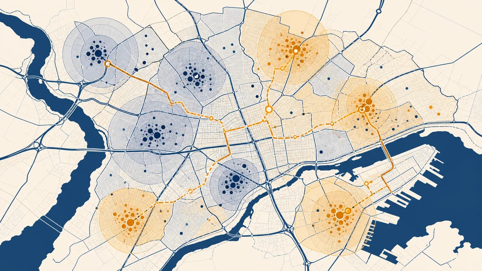
Spatial analysis is a set of geographic methods that measures patterns, relationships, and change according to location, in the context of places and processes on Earth. It answers common questions such as what spatial analysis means, how spatial data is analyzed, and how GIS spatial analysis finds clusters, routes, boundaries, and areas of influence. The idea exists because the location of an event can help explain why it happened, who it affects, and what may happen nearby.
A table can show that five neighborhoods have different numbers of bus stops. Spatial analysis adds coordinates, street connections, walking distance, population, and barriers such as rivers. It can then test which homes are poorly served, rather than simply ranking neighborhoods by stop count. Location becomes evidence.
What spatial analysis actually is
Spatial analysis is the examination of geographic features by their positions, shapes, attributes, and relationships. It asks where features occur, how they are arranged, what lies near or inside them, how they connect, and how those facts relate to a real process.
A feature is something represented in geographic data. A fire hydrant might be a point, a road a line, and a floodplain a polygon. Each feature can carry attributes. A road line might have a name, speed limit, surface type, and traffic count. Spatial analysis combines those attributes with geometry.
The word spatial means that position or arrangement matters. If a spreadsheet lists the addresses of clinics and schools, it contains location information, but it does not yet reveal a spatial relationship. Geocoding the addresses into coordinates allows an analyst to measure the distance between each school and clinic. Adding a street network makes it possible to calculate an actual route instead of a straight line.
Location is more than a coordinate. A useful location may also include which district contains it, which road connects to it, what lies uphill, and how long it takes to reach.
Spatial analysis is part of a wider set of geographic questions about human activity, physical systems, regions, and change. The geography concepts that connect places and processes show why location is treated as an explanatory variable rather than a label.
How spatial analysis works
Spatial analysis works by translating a geographic question into measurable relationships, preparing location data, applying a suitable operation, and checking the result against reality. The method must match the process: walking access needs routes, while flood exposure needs elevation and water movement.
Suppose a town wants to choose a site for a new emergency shelter. The question is not simply, “Where is empty land?” A workable site must be outside the flood zone, close to a major road, large enough for the building, and accessible to the population it will serve. Each phrase becomes a spatial condition.
Name the decision, study area, time period, and unit of analysis. “Find suitable shelter parcels within the town boundary” is more precise than “study emergency access.”
Represent parcels as polygons, roads as connected lines, population as small-area counts, and the flood zone as a polygon or depth surface. The representation determines which measurements are possible.
Check missing values, dates, duplicates, coordinate systems, boundaries, and measurement units. Two layers that appear together can still be misaligned or describe different years.
Exclude parcels that intersect the flood zone, select parcels above the minimum area, measure road access, and estimate travel time from populated areas.
Inspect high-ranking sites, compare the result with local knowledge, vary uncertain thresholds, and record assumptions. A field visit may reveal a locked gate or unstable ground absent from the data.
These operations are often carried out in software that stores, combines, and analyzes geographic layers. The software can process thousands of features quickly, but it does not decide whether the question, data, or assumptions are sensible.
How spatial relationships become measurable
Spatial relationships become measurable when vague geographic words such as near, dense, connected, and clustered receive explicit definitions. Analysts express them through distance, direction, containment, adjacency, overlap, network connection, density, or statistical similarity across a stated area and scale.
Distance measures separation
Distance can mean a straight line, travel along a network, time, cost, or even effort. For points on a flat coordinate grid, straight-line distance follows the Pythagorean relation.
For points at (2, 3) and (8, 11), the distance is coordinate units.
That answer is exact for the stated coordinate grid, but it may not describe a trip. A river, railway, slope, one-way street, or missing bridge can make the traveled distance much longer. Network analysis represents intersections as nodes and road segments as edges, then finds a path according to length, time, toll, or another cost.
Containment and overlap connect layers
A point-in-polygon operation can assign each reported accident to a police district. An intersection operation can identify farms that overlap a drought zone. A buffer creates an area within a chosen distance of a feature, such as land within 500 metres of a river. These operations answer different questions, even if their outputs look similar on a map.
Density measures amount per area
Density standardizes a count by the size of the area that contains it. It lets an analyst compare unequal districts, provided the chosen denominator suits the question.
If 24 trees are counted in 3 hectares, the measured density is trees per hectare.
Density does not show the exact arrangement within the area. Twenty-four trees could be evenly spaced, packed into one corner, or split into several groups. Point-pattern methods and local density surfaces can preserve more of that arrangement.
Spatial analysis versus map reading
Map reading interprets symbols and patterns already displayed, while spatial analysis calculates or tests geographic relationships to produce new information. A reader may notice that crashes seem concentrated downtown; an analyst defines downtown, compares rates, tests clustering, and checks exposure such as traffic volume.
You identify symbols, estimate direction, compare visible areas, and describe a pattern. The evidence is mainly what the map displays.
You specify a relationship, calculate it from geographic data, test alternatives, and create a result that was not present in any single input layer.
The distinction is not a contest between simple and advanced work. Careful map reading often generates the question that analysis tests. Analysis then produces another map, table, or model that must be read critically. methods for designing maps that communicate clearly govern how that result is classified, symbolized, and explained.
Consider a map with large circles where many people were injured in road collisions. The circles could mark raw totals. A district with more residents, more roads, or more vehicle trips may have more injuries simply because more people are exposed. Dividing injuries by population answers one question; dividing them by distance traveled answers another. Visual concentration alone cannot choose the correct denominator.
How scale and resolution change the answer
Scale and resolution change a spatial result because patterns depend on the size of the study area, the units used to group observations, and the detail captured by the data. A cluster visible by county can disappear or split when examined by neighborhood.
Geographic scale can refer to the extent of a study or the level at which observations are grouped. Resolution is the smallest spatial detail represented or measured. A land-cover raster with small cells can show narrow hedges that a coarse raster merges into nearby fields. Small cells do not guarantee accuracy, but they permit finer distinctions.
The last value follows directly from area: one kilometre is 1,000 metres, so one square kilometre contains ten-metre squares. Finer resolution greatly increases the number of cells to store and process.
Grouping also changes patterns. Imagine four equal blocks with household counts of 2, 2, 18, and 18. Reporting all four preserves two low and two high values. Pairing each low block with a high block creates two districts of 20 households each, making them look identical. This is a simple example of how aggregation can hide variation.
Scale should follow the process. A continental climate pattern and shade beside one building require different data. An analyst who studies walking access needs street crossings and entrances, not only regional road lines. More detail is useful only if it measures the feature relevant to the question.
How spatial data quality controls the result
Spatial data quality controls the result through positional accuracy, attribute accuracy, completeness, time, consistency, and fitness for purpose. A precise calculation cannot repair a missing road, an outdated population layer, or coordinates recorded in the wrong reference system.
Coordinates only make sense within a coordinate reference system. Latitude and longitude describe positions on Earth using angular values. Projected systems transform the curved surface onto a flat grid, usually so measurements can be made in linear units over a chosen area. Every projection distorts some combination of area, shape, distance, or direction.
A neat overlay can still be wrong. Layers may line up on screen after automatic transformation while their dates, definitions, accuracy, or collection methods remain incompatible.
Time is part of spatial quality. Comparing a current bus network with an old population map can misidentify underserved districts. A satellite image taken after harvest cannot directly answer a question about crop cover during peak growth. The page on how sensors observe Earth from a distance explains why pixel size, wavelength, cloud, and acquisition time affect what can be detected.
Good metadata records who created the dataset, when it was collected, what each field means, which coordinate system it uses, and where its limitations lie. Validation compares the data or output with an independent source. That might involve field observations, higher-quality reference data, withheld samples, or reports from people who know the place.
How spatial analysis shows up in city planning
Spatial analysis supports city planning by measuring access, land suitability, development pressure, service coverage, and conflicts among land uses. Planners combine parcels, transport networks, population, hazards, and regulations to compare sites and anticipate who gains or loses from a decision.
A library authority must choose between two possible branches. Site A is near more residents by straight-line distance. Site B connects to more homes by safe walking routes because a railway blocks access to Site A. A network analysis changes the preferred site.
A basic service-area analysis begins with a network. Each street segment receives a travel cost, perhaps minutes on foot. Crossings, stairs, turn restrictions, and entrances affect connection. The algorithm expands outward from the library until the accumulated cost reaches a threshold. Population areas intersecting that reachable network can then be counted or estimated.
Suitability analysis combines several criteria. A planner might exclude protected land, flood-prone parcels, and lots that are too small. The remaining parcels can be scored for transit access and proximity to the population. Exclusion rules and preference scores should remain separate. A parcel inside a prohibited zone is not rescued by having a high access score.
Equity requires looking beyond the total number served. A site that reaches the largest population may leave a smaller, isolated community without any service. Analysts can compare access by age, income, disability, or another relevant characteristic when lawful, ethical, sufficiently detailed data exists. The result informs a public decision; it does not replace public reasoning.
How spatial analysis shows up in health, hazards, and ecology
Spatial analysis connects health events, hazards, and ecological observations to possible sources, pathways, exposures, and vulnerable places. It can reveal where cases concentrate, model what lies downstream, estimate habitat connections, and direct limited fieldwork toward locations where evidence is most needed.
Disease mapping separates cases from risk
A map of case counts shows where recorded cases live or occurred. It does not automatically show where individual infection happened, nor does it measure risk. Population at risk, reporting practices, time, movement, and privacy all matter. Analysts commonly compare rates for areas, examine changes through time, and test possible relationships with care.
The famous 1854 Broad Street cholera investigation in London is a well-documented early example of mapping deaths near a water pump. The map supported a water-source explanation alongside interviews and local observation. Its lesson is methodological: location can expose a pattern, but causal conclusions need evidence about the mechanism.
Hazard models follow physical processes
Flood analysis may combine elevation, drainage, soil, rainfall, river channels, and buildings. A simple buffer around a river identifies proximity, but water does not spread equally in every direction. It follows terrain and connections. Wildfire and air-pollution models likewise require wind, fuel, topography, or atmospheric conditions rather than distance alone.
Ecological analysis measures habitat structure
Ecologists use spatial analysis to measure habitat area, edge, fragmentation, and connections between patches. Two forests with equal area can function differently if one is continuous and the other is divided by roads. Cost surfaces can represent how difficult each cell is for an animal to cross, allowing possible corridors to be compared.
Two observations occur near each other. This is a measured spatial association and may guide further investigation.
One process produced the other. This needs a plausible mechanism, timing, comparison, and evidence that competing explanations do not fit better.
Spatial association is useful without being proof of cause. A cluster of asthma cases near a busy road could reflect air pollution, but it could also be influenced by population density, housing, age, access to diagnosis, or where records were collected. The next analysis should distinguish these explanations.
What kinds of spatial analysis are most common
Common spatial analyses include queries, overlays, buffers, density estimates, interpolation, terrain calculations, network routes, cluster tests, and change detection. Each operation answers a distinct geographic question, so the method should be chosen from the question rather than from the available software menu.
| Question | Typical operation | Output |
|---|---|---|
| What is inside this area? | Point in polygon or spatial join | Features assigned to zones |
| What is within a set distance? | Buffer and intersection | A proximity zone or selected features |
| Where do two conditions coincide? | Overlay | Areas sharing specified properties |
| What is the least-cost route? | Network or cost-path analysis | A route and accumulated cost |
| What might values be between samples? | Interpolation | A continuous estimated surface |
| Where has the surface changed? | Raster comparison or image classification | Mapped categories or amounts of change |
Interpolation deserves special caution. It estimates values at unsampled locations using measured values nearby and assumptions about spatial continuity. A rainfall surface between gauges can be useful because rainfall varies across space, but the estimate becomes less certain where gauges are sparse or terrain changes sharply. Interpolation predicts a surface; it does not create observations.
Cluster analysis also needs a reference expectation. Ten incidents close together might look unusual, yet the pattern may be ordinary if nearly all people and streets occupy that small area. A statistical cluster method compares the observed arrangement with a defined alternative, often while accounting for the distribution of opportunities or population.
How can you tell if a spatial conclusion is reliable?
A spatial conclusion is reliable when its data fit the question, its method represents the real process, its assumptions are visible, and its result survives reasonable checks. Reliability increases when independent evidence agrees and decreases when small changes in boundaries or parameters reverse the answer.
Start by tracing the result backward. Which observations produced it? How were locations measured? What dates do the layers represent? Which records were excluded? Then inspect the model. A 10-minute drive-time area is only as credible as its road speeds, turn restrictions, and traffic assumptions.
Sensitivity analysis repeats the calculation with reasonable alternatives. If a proposed clinic site ranks first with a 15-minute travel limit but last with a 16-minute limit, the ranking is fragile. If it remains near the top under several plausible speeds, population estimates, and boundary choices, the conclusion is more stable.
Reproducibility is a practical test. Another analyst should be able to obtain the same output from the stated data, steps, parameters, and software settings.
Uncertainty should appear in the result rather than being hidden. A predicted pollution surface can show uncertainty alongside estimated concentration. A habitat corridor can be presented as one plausible route under stated movement costs, not as the path animals will certainly take. Honest limits make an analysis more useful because decision-makers can see what further evidence would change it.
Four mistakes people make with spatial analysis
Most spatial-analysis errors come from treating a convenient representation as if it were the place itself. Four recurring mistakes are confusing correlation with cause, using the wrong distance, ignoring scale and denominators, and trusting software output before checking data and assumptions.
1. Treating nearby events as proof of cause
Co-location suggests a question, not a verdict. An analyst should test time order, exposure, plausible pathways, competing explanations, and a comparison group. A source cannot explain events that occurred before it existed, and a visible cluster may simply follow where more people live.
2. Using straight-line distance for a network problem
People, vehicles, water, and animals move through different structures. Straight-line distance may be suitable for radio range under simplified conditions, but it can badly represent a walk across a divided highway. Use the distance or cost that follows the movement being studied.
3. Comparing counts without exposure or scale
A large district can contain more events because it contains more people, road, forest, or observation effort. Select a denominator that represents the opportunities for the event. Then check whether grouping at another reasonable scale changes the pattern.
4. Accepting clean output as accurate output
Software will calculate with incomplete, mistimed, or misprojected data. Inspect unusual records, compare the map with known landmarks, review metadata, and validate samples. A polished map can make an unsupported conclusion look more certain than it is.
Spatial analysis turns geography into testable evidence
Spatial analysis turns geography into testable evidence by connecting location, distance, shape, scale, and movement to questions about real places. Its strongest conclusions explain both the visible pattern and the process that could have produced it, while keeping uncertainty and alternatives in view.
The next time a map claims that an area is a hotspot, underserved, suitable, threatened, or accessible, look for the operation beneath the label. Ask what was counted, where the boundary came from, which distance was used, what date the data represents, and which comparison makes the pattern unusual.
The takeaway: Spatial analysis does not ask only where something is. It measures how location changes the answer, then checks whether the measurement matches the geographic process.
That habit connects the topic to geography as a whole. Places are shaped by physical conditions and human decisions, and both vary across space. Choose one claim on a map you see this week, identify its implied spatial relationship, and decide what evidence would test it.