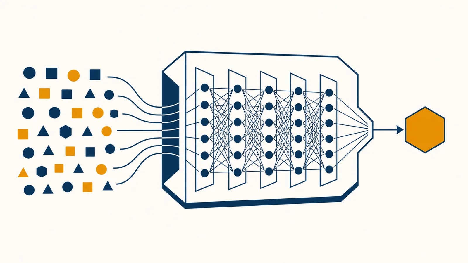
Machine learning is a method of computer programming that builds models from data so they can make predictions or decisions, in the context of artificial intelligence and data analysis. Put plainly, machine learning teaches computers to learn patterns from examples instead of requiring a programmer to write every rule. It exists because many useful tasks, such as recognizing speech, filtering spam, and estimating demand, involve patterns too numerous or changeable to list by hand. A machine learning model turns past observations into a rule that can handle a new observation, but only within the limits of its data, objective, and design.
What machine learning actually is?
Machine learning is a way to produce a prediction rule by fitting a mathematical model to examples. The model receives inputs, calculates an output, compares that output with evidence, and adjusts its internal parameters to reduce future error.
The word learning does not mean that the computer understands a lesson as a person does. It means that an algorithm changes stored numbers called parameters in response to data. Those numbers control how strongly different parts of an input affect the output. Once training ends, the resulting model can process an example it has not seen before.
Consider an email filter. Each message supplies input data, such as its words, sender information, and links. During training, known examples also carry labels such as spam or not spam. The algorithm searches for parameter values that make its predictions agree with those labels. After training, the model estimates the probability that a new message is spam.
This distinction separates the three main objects involved. Data supplies experience. A training algorithm changes parameters. A model is the fitted prediction rule left behind. People often call all three “the AI,” but keeping them separate makes a system easier to inspect and repair.
Training is not the same as using. Training estimates the model's parameters from examples. Inference uses those fixed parameters to produce an output for a new input.
How does a model learn a pattern from data?
A model learns by making a prediction, measuring how wrong it is, and changing its parameters in a direction that reduces that error. Repeating this cycle over many examples gradually fits a useful mapping from inputs to outputs.
Turn each case into values the model can accept, such as house size, number of rooms, and sale price.
Run the input through the current model. Early predictions may be poor because the parameters begin with unhelpful values.
Use a loss function to turn the gap between prediction and target into a number the algorithm can minimize.
Change the parameters according to how each one affected the loss. Gradient descent is a common update method.
Process more examples, then test performance on separate data to see whether the pattern carries beyond the training set.
A small model makes the mechanism visible. Suppose a shop wants to estimate the number of cold drinks sold from the afternoon temperature. It chooses a straight line:
If , , and the temperature , the model predicts drinks.
The hat over marks a prediction. The weight controls the slope, and the bias shifts the whole line. If the shop actually sold 76 drinks, the error is 6. A squared-error loss makes that error . Squaring prevents positive and negative errors from cancelling and penalizes larger misses more heavily.
Gradient descent asks how a small change in each parameter would change the loss. It then moves each parameter a small distance in the improving direction. The learning rate sets the step size. A rate that is too large can leap past a good solution; a rate that is too small can make training needlessly slow.
How do training, validation, and testing protect the result?
Training data fits the parameters, validation data guides choices about the model, and test data estimates final performance on unseen cases. Keeping these roles separate reduces the chance of mistaking memorization or repeated tuning for genuine predictive ability.
Imagine 1,000 labeled messages. A simple split could assign 700 to training, 150 to validation, and 150 to testing. Those numbers are an illustrative allocation, not a universal rule. The important condition is that the test examples remain untouched until design choices have finished.
A model that performs well on training data but poorly on new data is overfitting. It has captured details peculiar to its training set, perhaps even noise, rather than a pattern that generalizes. A model that performs poorly even on training data is often underfitting. Its form may be too simple, its features uninformative, or its training incomplete.
Validation data helps choose settings that training does not directly learn, called hyperparameters. Examples include tree depth, regularization strength, and the learning rate. If a team tries enough designs against the same validation set, it can overfit that set too. The final test set provides a cleaner check because it did not steer those choices.
Data leakage can make a weak model look excellent. Leakage occurs when training includes information that would not exist at prediction time, or when copies and close relatives of test cases appear in training.
Time matters as well. To predict next month's sales, a random split can accidentally train on later records and test on earlier ones. A time-based split, with older records used to predict newer records, better matches the intended use.
Supervised learning versus unsupervised learning versus reinforcement learning
Supervised learning fits inputs to known targets, unsupervised learning searches for structure without target labels, and reinforcement learning improves actions through rewards. The methods answer different questions, even though all use data to change a model or policy.
Supervised learning predicts a supplied target
Supervised learning trains on paired examples: an input and the answer associated with it. Classification predicts a category, such as fraudulent or legitimate. Regression predicts a quantity, such as travel time. The target supplies a direct signal for calculating error.
Unsupervised learning organizes unlabeled examples
Unsupervised learning receives inputs without answer labels and looks for useful structure. Clustering can group similar customers or documents. Dimensionality reduction can compress many measurements into fewer coordinates. A discovered cluster is a mathematical grouping, not automatically a meaningful human category.
Reinforcement learning improves a sequence of actions
Reinforcement learning trains an agent that observes a state, takes an action, and receives a reward. The challenge is that an action can affect rewards much later. A game-playing system may sacrifice a piece now because the resulting position improves its chance of winning.
Given past loan applications and known repayment outcomes, estimate the chance that a new applicant repays.
Given application records without repayment targets, find groups with similar financial profiles for investigation.
Many systems combine methods. A speech model might first learn general sound representations without hand labels, then receive supervised training on transcribed recordings. The surrounding field of turning raw data into defensible decisions also includes collection, cleaning, analysis, and communication, tasks that remain necessary regardless of the learning method.
How do features and representations determine what a model can see?
A feature is an input value exposed to a model, and a representation is the complete numerical form of an example. These choices determine which distinctions the model can detect, so weak or misleading representations limit even powerful algorithms.
A table might already contain usable features such as age in years, account balance, and number of recent purchases. Text, images, and sound require conversion into numbers. A simple text classifier can count words. An image model can process pixel values. An audio system can use measurements of sound energy across time and frequency.
Older machine learning projects often relied heavily on feature engineering, where people designed measurements they expected to matter. A spam detector might count links, capital letters, or known phrases. Deep learning can learn layered representations directly from rawer inputs. Early layers in an image network may respond to edges; later layers combine those signals into textures, parts, and task-specific patterns. how neural networks build layered representations explains that mechanism in detail.
A hiring model receives years of experience but not the kind of work performed. Two applicants with five years each look identical on that feature, even if one has direct experience with the role. The model cannot recover a distinction that the representation erased.
Encoding can also introduce false relationships. If a system represents city names as London = 1, Nairobi = 2, and Seoul = 3, an ordinary numerical model may treat Seoul as farther from London than Nairobi is. One-hot encoding avoids that ordering by giving each city its own indicator, though other methods are preferable when there are many possible values.
Missing values deserve an explicit policy. Zero may mean none, while a blank may mean unknown, not measured, or not applicable. Silently turning every blank into zero changes the claim made by the data. Good pipelines preserve that distinction and apply the same transformations during training and inference.
How does machine learning show up in real settings?
Machine learning appears wherever repeated data can support a useful prediction, ranking, detection, or generation task. Its output usually sits inside a larger system that collects inputs, applies rules, presents results, and lets people act or intervene.
Hospitals use predictions to direct attention
A model can highlight an image region, estimate the risk of deterioration, or prioritize records for review. The prediction does not arrive alone. Clinicians need information about the patient, the conditions under which the model was tested, and the consequences of false alarms and missed cases. A probability can support a decision without making the decision by itself.
Banks and shops score events as they happen
Fraud systems compare a new transaction with patterns in past activity. Useful inputs can include amount, time, merchant type, and recent account behavior. The system might approve the payment, request another check, or send it for human review. Attackers adapt, so the input distribution changes and performance must be monitored.
Search and recommendation systems rank choices
A ranking model estimates which results a person is likely to find useful. It may learn from queries, clicks, purchases, skips, and explicit ratings. Those observations are imperfect signals. A click can reflect curiosity or a misleading headline, while an unclicked result may simply have appeared too low on the page.
Language and vision systems process unstructured data
Models can classify documents, transcribe speech, locate objects, and generate text or images. These tasks differ in their outputs, but they share numerical representations and fitted parameters. The mechanics of how machines represent and process human language show why fluent text is still a prediction produced from patterns.
That separation matters in ordinary life. A keyboard model predicts the next word, but interface code decides which suggestions appear. A navigation model estimates travel time, but routing code compares possible paths. A streaming service predicts interest, while product rules determine what content is eligible to be recommended.
How should model performance be measured?
Model performance should be measured with a metric that matches the real cost of errors, on data that represents intended use. Accuracy alone can hide failure, especially when one outcome is rare or different mistakes carry unequal consequences.
A confusion matrix counts four outcomes for a binary classifier. A true positive is correctly flagged. A true negative is correctly cleared. A false positive is wrongly flagged. A false negative is wrongly cleared. Precision asks how many flagged cases were truly positive. Recall asks how many truly positive cases were found.
If 20 flagged messages contain 15 spam messages, precision is . If there were 25 spam messages in total, recall is .
Changing a classification threshold trades one kind of error for another. Suppose a model outputs a spam probability. Marking a message as spam above 0.50 will usually flag more messages than using 0.90. The lower threshold may catch more spam, increasing recall, but it can also trap more legitimate mail, reducing precision.
Regression uses measures suited to numerical differences. Mean absolute error averages the size of each miss without regard to direction. Mean squared error gives larger errors extra influence because it squares them. A delivery service may care about typical error, severe delays, or both, so it might report several measures and inspect performance across routes and times.
Baseline first. A sales model should beat a simple comparison, such as predicting the previous week's sales. A complicated model that loses to that baseline has not earned its complexity.
What five mistakes do people make with machine learning?
Common mistakes are treating correlation as cause, trusting a single score, ignoring biased samples, assuming deployment data will stay fixed, and confusing fluent output with factual knowledge. Each mistake turns a limited prediction tool into a stronger claim than evidence supports.
1. They read causation into prediction
A model can discover that two variables move together without showing that one causes the other. Ice cream sales and sunburn cases may rise together because hot, sunny weather affects both. A predictor can exploit that relationship, but changing ice cream sales would not therefore control sunburn. Causal claims need a suitable experiment or a defensible causal design.
2. They report one average score
An overall result can conceal different performance across locations, device types, or groups of people. A voice system tested mostly in quiet rooms may struggle in traffic. Breaking results into relevant slices reveals where a model works and where the evidence is thin.
3. They treat available data as representative data
A dataset reflects how records were collected. A survey of app users omits nonusers. Historical arrests reflect policing patterns as well as crime. Labels may encode human disagreement or old policy. More rows do not correct a sample drawn from the wrong population.
4. They assume the future matches the past
Distribution shift occurs when the data encountered after deployment differs from training data. New slang can weaken a moderation model. A new sensor can change measurements. Monitoring should track input changes, missing values, errors, and outcomes after release.
5. They mistake confidence for knowledge
A model's probability or fluent wording comes from its learned mapping, not from a guarantee of truth. Confidence can be poorly calibrated, particularly on unfamiliar inputs. High-stakes systems need checks, sources where applicable, and a safe way to abstain or request review.
“The model is 95 percent accurate, so its decisions are reliable.”
“On this stated test set, it made 950 correct classifications out of 1,000. Here are the error types, subgroup results, and test conditions.”
The 95 percent in this comparison follows from the shown arithmetic. It still cannot tell us whether the errors are acceptable. Missing five dangerous cases may matter more than falsely flagging forty-five safe ones, or the reverse, depending on the task.
How much data does machine learning need?
Machine learning needs enough relevant, representative examples to constrain the chosen model, but there is no universal minimum. The required amount depends on task variety, label quality, model complexity, acceptable error, and how much prior training the model already has.
A straight-line model with two parameters can be estimated from a small clean dataset, though more observations help measure uncertainty. An image classifier expected to recognize many objects under varied lighting, angles, and backgrounds faces a much larger problem. It must encounter enough variation to separate the stable signal from accidental details.
Quality often beats unexamined volume. Duplicate records make a dataset look larger without adding much information. Incorrect labels teach the wrong mapping. A million examples from one camera may not prepare a model for another camera with different color and resolution. Before collecting more rows, teams inspect coverage, label consistency, missing cases, and the gap between recorded examples and intended use.
Transfer learning changes the calculation. A model already trained on broad data can be adapted to a narrower task with fewer new examples because many useful representations are already present. The new dataset still has to cover the distinctions that matter locally.
Can a machine learning model explain its decision?
Some models expose their reasoning structure directly, while others require approximate explanation tools. An explanation can show which inputs influenced an output, but it does not prove causation, fairness, correctness, or that the model would behave similarly elsewhere.
A small decision tree can be read as a sequence of tests. A linear model exposes a coefficient for each feature, although correlated features can make those coefficients hard to interpret. A large neural network spreads information across many parameters, so people often use methods that perturb inputs, attribute importance, or compare a case with similar examples.
Explanation has several meanings. A developer debugging a model may need feature contributions. A person denied a service may need the specific factors and an actionable appeal process. An auditor may need training records, evaluation results, and change history. One colorful feature chart cannot satisfy all three needs.
An explanation describes model behavior, not reality itself. If a model relies on postcode, an attribution method may reveal that reliance. It cannot by itself establish that postcode is a fair or causal basis for the decision.
Can machine learning keep learning after deployment?
A deployed model can be updated with new data, but safe updating requires fresh labels, evaluation, version control, and rollback. Most production systems retrain in controlled batches rather than changing instantly after every interaction because feedback can be noisy or manipulated.
Online learning updates a model as observations arrive. It is useful where patterns change quickly or storing all past data is impractical. It also creates risks. A faulty sensor can corrupt many updates, and coordinated users can feed adversarial examples. Delayed outcomes make it hard to know which predictions were actually correct.
Batch retraining offers a checkpoint. A team gathers new data, checks it, trains a candidate, compares that candidate with the current model, and releases it only if it passes defined tests. Model and dataset versions allow the team to trace which code and evidence produced any prediction.
A grocery demand model was trained during ordinary weeks. A holiday changes buying patterns, so forecast errors climb. Monitoring detects the change. Staff can switch to a seasonal model, add holiday features, or temporarily rely more on human ordering instead of assuming the original fit still applies.
Machine learning turns computer science into testable prediction systems
Machine learning connects algorithms, data structures, probability, software engineering, and human judgment in one testable system. Its central discipline is simple: define the task, measure error on relevant evidence, and keep checking after the code meets reality.
A trained model is still software. It needs input validation, efficient storage, access controls, tests, interfaces, logs, and maintenance. Its data has a schema. Its predictions travel through programs. Its failures interact with people and institutions. The broader set of computer science concepts behind working digital systems explains why model training is only one part of building something dependable.
The next time an app ranks a result, completes a sentence, flags a payment, or identifies an object, look for four things: the examples it could have learned from, the target it was trained to optimize, the errors its metric rewards or hides, and the action surrounding software takes. Those questions turn “AI” from a vague label into a system you can examine.
The takeaway: Machine learning does not replace programmed logic with magic. It replaces some hand-written rules with parameters fitted from data, then relies on computer science to test, deploy, monitor, and govern the resulting behavior.