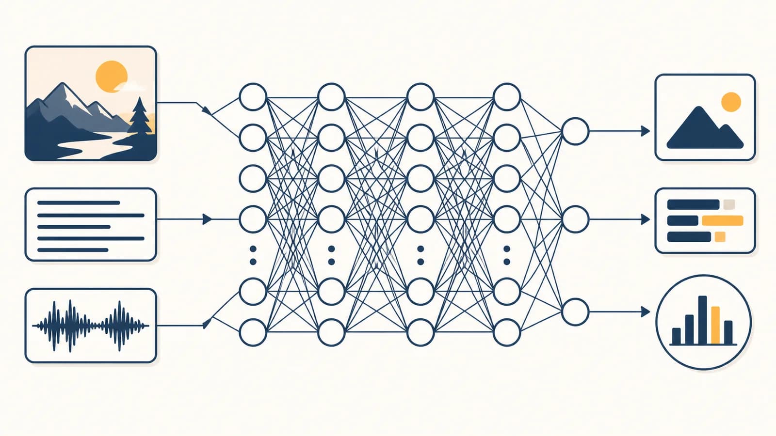
Deep learning is a machine-learning approach that trains layered neural networks to transform examples into predictions or generated content, in the context of artificial intelligence. A neural network can learn to recognize images, process text, and generate speech because its adjustable connections capture patterns in training data. Deep learning means using networks with many processing layers. The idea exists because programmers cannot write a complete rulebook for every face, sentence, sound, or unusual case a computer may meet.
Give a conventional program a photograph and it receives millions of color values, not a ready-made label such as “bicycle.” A learned model turns those values into useful evidence. Early layers may respond to edges. Later layers combine edges into curves, parts, and eventually a probability for each possible label. The machine does not see as a person sees. It performs numerical operations whose results happen to support useful decisions.
What a neural network actually is
A neural network is a function built from connected units arranged in layers. Each unit combines incoming numbers, adds an adjustable bias, and applies an activation function. Training changes the weights and biases so the network maps selected inputs to useful outputs.
The name comes from a loose comparison with biological neurons, but the mathematical object is much simpler than a brain cell. A unit receives a vector of inputs. It multiplies each input by a weight, sums the results, adds a bias, and passes the total through a function. One unit can be written as:
If the inputs are 2 and 3, the weights are 0.5 and -1, and the bias is 1, the value before activation is .
The weights control which inputs matter and in which direction. A positive weight makes a larger input push the result upward. A negative weight pushes it downward. The bias shifts the threshold at which a unit responds. The activation function adds nonlinearity, which lets stacked layers describe curved and complicated boundaries instead of collapsing into one large linear calculation.
A whole layer processes many units at once. In matrix notation, the calculation is compact:
The input vector is multiplied by the weight matrix , shifted by , then transformed element by element by .
The word architecture means the planned arrangement of layers and connections. The word parameters means the numbers learned during training, mainly weights and biases. The architecture is like the shape of an empty spreadsheet; the parameters are the filled cells that determine what the finished calculation does.
How deep learning works
Deep learning works by passing an input forward through several layers, measuring the output against a target, sending error information backward, and adjusting parameters to reduce future error. Repeating this process across many examples gradually produces a useful input-to-output function.
Suppose a small network must classify a picture as a cat or a dog. During a forward pass, pixel values enter the first layer. Each later layer transforms the previous layer’s output. The final unit might produce 0.80 for “cat,” interpreted as the model’s current estimated probability under its setup.
If the correct label is dog, the prediction is poor. A loss function converts that mismatch into a number. Cross-entropy loss is common for classification because it strongly penalizes confident wrong answers. If the target class has predicted probability , its loss for that example is:
A correct-class probability of gives about ; a probability of gives about . Lower is better.
Next comes backpropagation. Calculus provides a gradient for every parameter: a local estimate of how changing that parameter would change the loss. The chain rule carries this information backward through the layers. It does not assign human explanations to units. It efficiently computes responsibility within a long composition of functions.
Convert examples into numerical tensors and pair them with labels, next tokens, or another training target.
Apply every layer in order to produce predictions from the current parameter values.
Use a defined score to measure how far the predictions are from the training targets.
Apply the chain rule to calculate how each parameter contributed to the loss.
Move weights a small distance in a direction expected to reduce loss, then repeat with another batch.
A basic gradient descent update is . The learning rate sets the step size. A rate that is too large can jump past good solutions. One that is too small can make learning slow or leave the model stuck near an unhelpful region. Practical optimizers such as Adam modify the update using recent gradient behavior, but they still depend on the same central signal.
Training, validation, and testing have different jobs
The training set supplies examples used to update parameters. The validation set guides choices such as architecture, learning rate, and stopping time. The test set estimates performance only after those choices are settled. Repeatedly checking the test set and redesigning the model around it quietly turns that test data into another validation set.
This distinction protects against overfitting, the condition in which a model learns training details that do not generalize. A model might memorize backgrounds in a small animal dataset, then fail when the same animals appear indoors. Good test examples must represent the conditions in which the system will actually operate.
Neural networks versus ordinary programs
An ordinary program follows rules written directly by a programmer, while a neural network learns parameter values from examples within an architecture chosen by people. Both execute exact instructions on hardware, but the source of their decision logic and their failure patterns differ.
A developer writes conditions such as “if the account balance is below the withdrawal, reject the transaction.” The rule is inspectable, stable, and suitable when requirements can be stated precisely.
A training process adjusts parameters after seeing examples. The result can handle patterns that resist hand-written rules, but it can also absorb hidden biases and shortcuts from the data.
Use arithmetic code to calculate tax under a published formula. Use a database query to look up an exact account. A neural network is a better candidate when inputs are messy and the desired pattern is difficult to specify, such as recognizing speech through background noise. Many useful systems combine both approaches. A model reads a document; conventional code checks permissions, records the result, and applies fixed business rules.
Deep learning is also narrower than machine learning. Decision trees, linear regression, nearest-neighbor methods, and support vector machines can learn from data without deep networks. The broader relationship is explained in how computers learn patterns from data. Neural networks are one family inside that larger field, and deep neural networks are a large, layered part of that family.
Learned does not mean self-directed. People choose the data, objective, model architecture, evaluation method, and deployment rules. The training algorithm searches for parameter values inside those choices.
How neural networks see images
Image networks see by converting pixel arrays into feature maps and combining local visual patterns across layers. Early calculations detect simple contrasts and textures; later calculations assemble spatial evidence into objects, regions, captions, or pixel-level outputs for a defined task.
A color image is commonly stored as a grid with red, green, and blue channel values. A 224 by 224 image with three channels contains input values. The network receives this tensor. It does not initially receive “wheel,” “shadow,” or “pedestrian.”
A convolutional layer slides a small learned filter across the grid. At each position, it multiplies nearby pixel values by filter weights and sums them. Because the same filter is reused across positions, it can respond to a pattern wherever that pattern appears. A vertical-edge filter that activates on the left side of a frame can also activate on the right.
A phone camera app tries to isolate a person for background blur. A segmentation network produces a class prediction for each pixel. The app then uses conventional graphics code to keep person pixels sharp and blur pixels assigned to the background. Stray hair, glass, and low contrast make the boundary difficult.
Modern vision systems may also split an image into patches and process them with transformer layers. Attention lets one patch combine information from other patches, which helps connect separated parts of an object. Convolutions and vision transformers use different arrangements, but both turn raw arrays into successively more useful internal representations.
Classification answers “what category best fits this image?” Object detection also predicts bounding boxes. Segmentation assigns categories to pixels. Image generation starts with noise or another representation and constructs an image conditioned on text or other inputs. These tasks need different outputs and losses, even if they reuse similar learned components. The task boundaries and applications receive more detail in how machines extract meaning from images.
How neural networks read and write language
Language networks process text by turning pieces called tokens into vectors, mixing information across their context, and predicting useful outputs such as a label or the next token. Repeated next-token prediction can produce paragraphs, code, summaries, and structured answers one token at a time.
A tokenizer divides text into vocabulary entries. These may be whole words, punctuation marks, or word pieces. The exact split depends on the tokenizer. Each token ID selects an embedding, a learned vector of numbers. Similar uses can lead to related vector patterns, although no single coordinate is guaranteed to mean one human concept.
Transformers use attention to combine contextual information. For each token, the network produces query, key, and value vectors. Query-key similarity controls how much of each value contributes to the updated representation. A simplified single-head attention calculation is:
The softmax turns similarity scores into nonnegative weights that sum to 1 for each query, then those weights mix the value vectors.
Consider “The trophy did not fit in the suitcase because it was too large.” To form a useful representation of “it,” attention can draw on “trophy,” “suitcase,” “fit,” and “large.” Different attention heads can learn different patterns. Later feed-forward layers transform each position further. Position information is also added because attention alone does not know word order.
A language model is commonly trained to predict a hidden or next token using text examples. During generation, it produces a probability distribution over possible next tokens, selects one according to a decoding rule, appends it, and repeats. The generated sentence is therefore a sequence of conditional choices, not a paragraph retrieved whole from a secret drawer.
Next-token training can capture grammar, style, facts expressed in training text, and patterns of reasoning demonstrations. It does not install a guaranteed fact database. A fluent model can continue a false premise or produce a plausible detail that its calculations do not support. Retrieval systems can supply documents, and tools can perform calculations, but the application must still check sources and tool results. the methods computers use to work with text places language models alongside search, classification, translation, and information extraction.
How neural networks hear and speak
Speech networks turn changing air-pressure measurements into numerical time series, extract patterns across time and frequency, and map those patterns to text or audio. Speech recognition predicts language from sound, while speech synthesis predicts acoustic content that a waveform generator can render as sound.
A microphone samples air pressure at regular intervals. Raw waveform samples contain timing detail, but many systems first calculate a spectrogram, which describes how energy at different frequency bands changes over time. Spoken vowels create characteristic frequency patterns. Consonants may produce brief bursts or noisy bands. The network learns associations between these acoustic structures and linguistic units.
Automatic speech recognition must handle more than individual sounds. The same sound can belong to different words, speakers pronounce sounds differently, and background noise hides evidence. Context can favor one transcript over another. A model may combine an acoustic representation with a language representation so that both the recording and likely word sequences influence the result.
During a video call, live captions receive short audio chunks, estimate words, revise recent guesses as more context arrives, and display text under a delay limit. Names, code-switching, crosstalk, and a weak microphone create predictable trouble. A confident caption can still be wrong.
Text-to-speech usually begins with text units and predicts an acoustic representation, such as a spectrogram or learned audio code. A vocoder or decoder converts that representation into a waveform. A voice-cloning system may condition generation on a speaker embedding derived from a reference recording. This creates useful accessibility tools and serious impersonation risks, so consent, labeling, and identity checks matter in deployment.
How deep learning shows up in real decisions
Deep learning appears in decisions whenever software classifies messy inputs, ranks alternatives, generates content, or detects unusual patterns. Its output is often one component in a larger process involving databases, fixed rules, human review, security checks, and consequences outside the computer.
A warehouse camera can flag damaged packages. A bank can use a learned model as one signal in transaction monitoring. A hospital imaging system can mark regions for a clinician to inspect. A search service can rank documents by estimated relevance. A car can estimate lanes and nearby objects. A creative tool can propose an image or remove background noise.
The important unit of evaluation is the full decision process, not only the model. A classifier can have a good average test score and still fail badly for a rare class. It can also be placed behind a poor threshold. If a safety system turns a probability into an alert, lowering the threshold catches more possible cases but usually creates more false alarms. The acceptable trade depends on what a missed case and a false alarm each cause.
| Setting | Model output | What must also be checked |
|---|---|---|
| Medical image review | Region or risk score | Clinical context, scanner differences, false negatives, and qualified human judgment |
| Content moderation | Category probabilities | Language context, appeals, policy definitions, and uneven error rates |
| Fraud screening | Anomaly or risk score | Identity evidence, changing attacker behavior, customer impact, and review capacity |
| Search ranking | Relevance score | Source quality, freshness, user intent, manipulation, and diversity of results |
Dataset construction is part of system design. Labels can be inconsistent. Historical records can encode previous discrimination. Cameras can behave differently in rain or darkness. Text collected from one community may not represent another. Data scientists examine these gaps, design measurements, and connect model outputs to defensible decisions.
A high test score is conditional evidence. It supports performance only for examples, labels, and conditions represented by the evaluation. Deployment can change all three.
Once deployed, a model can affect the data later used to retrain it. A recommendation system promotes some items, so those items receive more clicks, which can then make them appear even more attractive. This feedback loop is a property of the surrounding system. Monitoring must therefore track input shifts, errors, complaints, overrides, and downstream outcomes rather than only server uptime.
4 mistakes people make with deep learning
Four common mistakes are treating neural networks as digital brains, confusing confident output with knowledge, testing on familiar data, and ignoring the surrounding system. Each mistake hides a different source of error, so each requires a different check or design response.
1. Calling every internal unit a human-like thought
A neuron is a mathematical calculation, and a hidden-layer activation is a number. Researchers can sometimes connect groups of activations to recognizable patterns, but assigning a neat concept to every unit overstates what is known. Representations are often distributed across many dimensions, and one unit may respond in several contexts.
2. Treating confidence as proof
A softmax score reports a model’s relative output under its calculation. It is not automatically a calibrated probability, a source citation, or evidence that the input resembles training data. Calibration testing compares predicted confidence with observed frequency. Source verification checks factual claims. Out-of-distribution testing asks what happens on unfamiliar inputs. These are separate jobs.
3. Letting test examples leak into training choices
Data leakage occurs when information unavailable at real prediction time reaches training or evaluation. A medical model might accidentally read a mark added after diagnosis. Duplicate photographs may appear in both training and test sets. A future event may be included in a feature used to predict the past. The score then measures access to leaked clues, not the intended ability.
4. Blaming or praising the model alone
People set the objective, select data, write interface text, choose thresholds, and decide when a person can appeal. A model may be accurate while an application uses its output irresponsibly. A weaker model can be useful inside a cautious workflow with clear limits. Responsibility belongs to the organizations and people operating the system, not to an equation.
More layers, more data, or a larger parameter count automatically makes a system better for every use.
Scale can improve capacity, but task fit, data quality, compute cost, response time, evaluation coverage, and error consequences determine usefulness.
What deep, hidden, and generative actually mean
Deep means that a network contains multiple successive representation layers, hidden means a layer sits between observed input and requested output, and generative means a model learns to produce or assign probabilities to data rather than only choosing a fixed class.
There is no single scientific boundary at which a network suddenly becomes deep. The word distinguishes layered representation learning from shallow models, but architecture matters more than the label. A residual network may contain many blocks with shortcut connections. A transformer repeats attention and feed-forward blocks. Counting layers can depend on which operations a writer chooses to count.
A hidden layer is not secret code. Its values are simply intermediate, neither the raw input nor the final output supplied for the task. Those values can be logged and studied. “Hidden” describes the layer’s place in the function.
A discriminative classifier estimates a label or boundary, such as spam versus legitimate email. A generative model represents how data can be produced, or predicts parts of data conditioned on other parts. Language models generate token sequences. Diffusion models learn to reverse a process that adds noise, allowing them to construct samples from noise through repeated denoising steps.
Deep learning is a method, not a product category. A chatbot, camera feature, laboratory tool, and music generator may all use deep networks while having different inputs, objectives, interfaces, and risks.
How much data and computing does a network need?
A network needs enough representative data and computing for its task, architecture, and accuracy target; there is no universal minimum. Small models can learn narrow patterns on modest datasets, while broad generative models require far greater resources and are often adapted rather than trained anew.
The required data depends on variation. Recognizing two clean symbols in a controlled image may need relatively few labeled examples. Recognizing street objects across countries, weather, cameras, and lighting requires examples covering those conditions. Ten near-duplicate images add less information than ten images that reveal distinct cases.
Compute is spent on tensor operations, mainly large matrix multiplications. Graphics processing units are useful because they can perform many related numerical operations in parallel. Memory also matters because training stores parameters, activations, optimizer state, and batches. Training generally costs more than running one prediction, called inference, because training includes the backward pass and repeated updates.
Transfer learning reduces the starting cost. A model trained on a broad source task can be fine-tuned on a smaller task-specific dataset. Sometimes the base parameters are frozen and only a small output layer or adapter is trained. The result still needs evaluation on the actual target population. Pretraining supplies a starting representation, not a guarantee.
Can anyone explain a neural network’s answer?
A neural network’s answer can often be investigated, but a complete human-readable explanation is rarely available for a large model. Interpretation methods reveal sensitivities, examples, and internal patterns; they do not automatically prove the cause, truth, fairness, or safety of a decision.
For an image classifier, a saliency map can estimate which pixels most affect a score. For a tabular model, feature attribution can estimate contributions relative to a baseline. For a language model, researchers can inspect attention patterns, activations, or the effect of changing words. Similar training examples can reveal what evidence the model may have reused.
Each method answers a specific question. A heat map can show where sensitivity is concentrated without showing why the model learned that sensitivity. An attribution can change when the baseline changes. Attention weights show information mixing inside one operation, but they are not a complete explanation of the final output. Counterfactual tests are often clearer: change one relevant feature while holding others steady and observe the prediction.
If a plant-disease classifier predicts “diseased,” cover the leaf, change the background, and test photos from another camera. If the prediction follows the table surface rather than the leaf markings, the model learned a shortcut. The experiment produces evidence that a colorful explanation graphic alone may miss.
High-impact uses need several kinds of evidence: task performance, subgroup analysis where appropriate and lawful, stress tests, documentation of data limits, human review, and a way to contest errors. Interpretability contributes to that evidence. It does not replace it.
Deep learning is applied computer science
Deep learning joins algorithms, data structures, numerical methods, hardware, software engineering, security, and human-computer interaction. Learning the equations explains the model, but understanding the full system requires tracing how inputs are collected, outputs become actions, and failures reach people.
A useful first exercise is small enough to inspect. Train a tiny classifier on two features, plot its decision boundary, and change one training example. Watch the boundary move. Then split the data properly, compare training and validation loss, and test an example unlike those in training. That sequence turns terms such as gradient, overfitting, and distribution shift into visible behavior.
Outside a classroom, notice where software makes a fuzzy judgment: a photo search, an automatic caption, a fraud alert, a translation, or a recommended song. Ask five concrete questions. What numbers entered the model? What target shaped training? What output did it produce? What rule turned that output into an action? Who can detect and correct an error?
The takeaway: A deep network is a layered, adjustable function trained by measured error. Its impressive behavior comes from learned numerical structure, while its reliability depends on data, evaluation, software, and the decisions built around it.
Those questions connect neural networks to the broader study of computation, including representation, algorithms, testing, and social consequences. Follow how these ideas fit across computer science, then choose one AI feature you use this week and trace its likely path from input to decision.