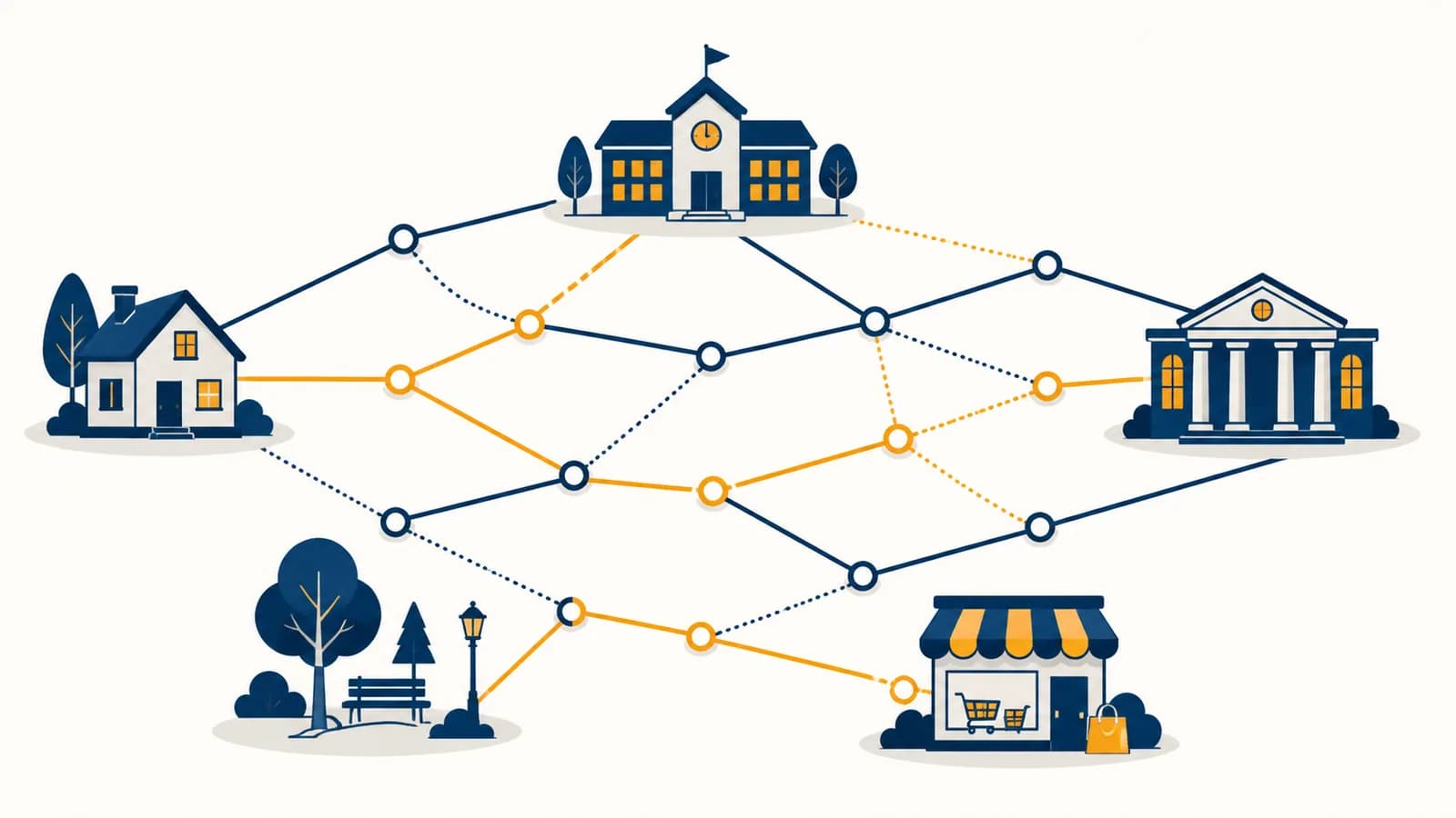
Graph algorithms are procedures that find routes, groups, rankings, and other patterns in networks of connected objects, in the context of computer science. A graph stores objects as vertices and relationships as edges. Graph traversal, breadth-first search, depth-first search, shortest path algorithms, Dijkstra's algorithm, minimum spanning trees, and topological sorting exist because many problems depend more on connections than on the objects themselves. A street map, a dependency list, and a social network look different, but each can become a graph and be processed by the same small set of ideas.
What a graph actually is
A graph is a data model made of vertices and edges: vertices represent things, while edges represent relationships between pairs of things. The meaning of each vertex and edge comes from the problem, so the same structure can describe roads, friendships, computer links, or prerequisites.
Suppose five places are labeled Home, Library, School, Park, and Shop. Draw a line whenever a direct road joins two places. The places are vertices, sometimes called nodes, and the roads are edges. A route from Home to School is a sequence of adjacent vertices, such as Home, Library, School. Its length may mean two edges, or it may mean the total travel time recorded on those edges.
Edges can carry more information than existence. A weighted edge might store distance, travel time, price, or capacity. A directed edge has an arrow, so an edge from A to B does not automatically allow movement from B to A. One-way streets and account follows are directed. A friendship is usually modeled as undirected because the relationship applies in both directions.
A path does not repeat edges unnecessarily and connects one vertex to another through successive edges. A cycle returns to its starting vertex. A connected component is a set of vertices that can reach one another, with no path to vertices outside the set. These definitions let an algorithm ask precise questions instead of treating a network as a vague picture.
A graph is not a chart. In graph theory, the word names a network of vertices and edges. A bar graph and a line graph display measurements, but they are not usually the graphs processed by graph algorithms.
How graph representation works
A graph representation turns vertices and edges into data a program can inspect. An adjacency list records each vertex's neighbors, while an adjacency matrix uses a grid whose cells state whether two vertices are connected, and sometimes records the edge weight as well.
For the roads Home to Library, Home to Shop, Library to School, and Shop to School, an adjacency list could store Home with Library and Shop, then Library with Home and School. In an undirected graph, each road appears in both endpoint lists. In a directed graph, an outgoing edge normally appears only in the source vertex's list.
| Representation | Storage | Checking one edge | Best fit |
|---|---|---|---|
| Adjacency list | Usually scans one neighbor list | Sparse graphs with relatively few edges | |
| Adjacency matrix | Dense graphs or frequent edge checks | ||
| Edge list | Usually scans edges | Algorithms that process every edge directly |
Here, is the number of vertices and is the number of edges. The big O expressions describe how storage grows, not the exact number of bytes. An adjacency matrix for 1,000 vertices has one million cells because , even if only a few thousand pairs are connected. An adjacency list stores only the connections that exist, plus bookkeeping.
The representation changes the cost of the algorithm. Breadth-first search examines the neighbor list of every reached vertex, so an adjacency list lets it cover a graph in time. With a matrix, it may inspect an entire row for every vertex, producing work. The algorithmic idea stays the same, but the data structure decides how quickly the next edge can be found. The guide to choosing lists, trees, maps, and other data structures develops this connection between storage and operations.
How graph traversal works
Graph traversal systematically visits reachable vertices while marking each one, so cycles do not cause endless repetition. Breadth-first search uses a queue to expand outward by distance in edges. Depth-first search uses a stack, often through recursion, to follow one branch before returning.
Put the start vertex in a queue and mark it discovered immediately. Marking on insertion prevents the same vertex from entering the queue through several neighbors.
Take the vertex at the front of the queue. Inspect its data if the task needs it, then read its outgoing neighbors.
For each unmarked neighbor, record its parent, mark it, and place it at the back of the queue. The parent links can later reconstruct a route.
An empty queue means every vertex reachable from the start has been processed. Unmarked vertices belong to another component or cannot be reached in the directed graph.
Run breadth-first search on Home, with neighbors ordered Library then Shop. The queue begins with Home. Removing Home adds Library and Shop. Removing Library adds School. Removing Shop does not add School again because School is already marked. School is therefore two edges from Home. Parent pointers might record School's parent as Library and Library's parent as Home, giving the path Home, Library, School.
The queue creates layers. Every vertex one edge from Home enters before any vertex two edges away. That is why breadth-first search finds a shortest path in an unweighted graph. If edges have different costs, the fewest edges may not give the least total cost, so a different algorithm is needed.
Traversal also solves reachability and component problems. A program can begin at one account and test whether another account is reachable, count islands in a grid by treating adjacent land cells as connected vertices, or label disconnected groups in a network. For a graph stored as adjacency lists, both breadth-first search and depth-first search take time because each vertex is marked once and each edge is inspected a bounded number of times.
Breadth-first search versus depth-first search
Breadth-first search explores vertices in expanding layers and is suited to minimum edge counts. Depth-first search follows a branch as far as possible before backtracking and is suited to structural questions such as cycle detection, dependency order, and connected region discovery.
A queue preserves discovery order. The search reaches all vertices at distance one, then distance two, and so on. It can return the fewest-hop path in an unweighted graph, but a wide layer may make the queue large.
A stack preserves the current branch. The search can record entry and exit times, expose back edges that signal cycles, and produce a dependency order. A long branch can make the explicit stack or call stack large.
Consider a maze where every legal move costs one step. Breadth-first search finds an exit using the fewest moves because it tests cells by distance. Depth-first search can find an exit, but the first exit found may lie at the end of a winding route. If the task is only to determine whether any exit exists, either method is valid.
The order among neighbors can change the exact traversal without changing correctness. If Home lists Library before Shop, Library is visited first. Reversing the list changes the visit order and may choose a different shortest path of equal length. Reproducible software often sorts identifiers or preserves a defined input order so tests do not depend on accidental storage details.
How shortest path algorithms work
A shortest path algorithm finds a route with minimum total edge cost between vertices. Breadth-first search handles equal-cost edges, Dijkstra's algorithm handles nonnegative weights, and Bellman-Ford can handle negative weights while also detecting reachable negative-cost cycles.
Dijkstra's algorithm maintains a tentative distance to each vertex. The start receives distance zero and every other vertex begins at infinity. A priority queue repeatedly selects the unsettled vertex with the smallest tentative distance. The algorithm then relaxes its outgoing edges, which means testing whether reaching a neighbor through this vertex gives a lower cost.
If Home to Library costs 4 and Library to School costs 3, a known distance of 4 to Library proposes to School.
Suppose Home to School directly costs 10, Home to Library costs 4, and Library to School costs 3. Starting at Home gives tentative values 10 for School and 4 for Library. The priority queue selects Library next. Relaxing Library to School replaces 10 with 7. When School becomes the smallest unsettled vertex, its distance is final under the nonnegative-weight condition.
A driver needs the quickest route, not the shortest distance. The graph uses intersections as vertices and road segments as directed edges. Each weight is an estimated travel time. A turn restriction removes an edge, while a one-way road contributes an edge in only one direction.
Dijkstra's guarantee depends on weights being nonnegative. Once the smallest tentative vertex is settled, a later route cannot improve it, because adding another nonnegative edge cannot reduce a path's cost. A negative edge breaks that logic. Bellman-Ford instead relaxes every edge repeatedly. After rounds, any shortest simple path has had enough rounds to propagate through at most edges. If one more round still improves a distance, a reachable negative cycle exists.
The A* algorithm can reduce work when searching toward one target. It ranks a vertex using cost already paid plus a heuristic estimate of cost remaining. For road distance, straight-line distance can be a useful lower bound. If the heuristic never overestimates the true remaining cost, A* can preserve optimality while directing attention toward the destination.
How graph algorithms show up in routes, networks, and software
Graph algorithms appear whenever a system must follow connections, choose a route, detect separation, or respect dependencies. Mapping software searches road graphs, network tools route packets, build systems order tasks, and games search spaces of positions and possible moves.
A map is more than dots joined by lines. Intersections may be split into several vertices to represent legal turns. Roads have direction, estimated time, restrictions, and sometimes changing conditions. A route request then becomes a shortest path query over a prepared graph. The displayed road line is only the visible surface of a data model built for legal movement.
Computer networks also form graphs, but the chosen objective depends on the layer and protocol. A router may select a path according to configured link costs, while diagnostic software can test reachability or identify a failed connection that splits part of a network. The word shortest therefore means lowest according to the system's metric, not automatically fewest physical metres.
Build tools model source files or tasks as vertices and prerequisites as directed edges. If task B needs the output of task A, the graph contains A to B. A topological order gives a legal execution sequence. Independent tasks can run concurrently, while a cycle such as A requiring B and B requiring A reports a dependency error rather than a usable order.
Games create graphs even when they do not store every vertex in advance. A puzzle state can be a vertex, and one legal move creates an edge to another state. Search generates neighboring states as needed. Pathfinding on a tile map treats walkable cells or navigation regions as vertices. The search then runs inside an update loop that must keep the interactive system responsive.
The model chooses the answer. If an edge weight records distance, the algorithm minimizes distance. If it records time, risk, or price, it minimizes that quantity. A correct algorithm can still answer the wrong real-world question when its graph is modeled badly.
How graphs produce rankings, groups, and recommendations
Graph methods can score important vertices, divide a network into groups, and propose new connections by using the pattern of edges. These results are inferences from a chosen model, so their meaning depends on what an edge records and what the method rewards.
A simple degree score counts incident edges. In a directed graph, in-degree counts incoming edges and out-degree counts outgoing edges. This may be useful, but it treats every connection alike. More involved ranking methods allow a link from a well-connected or highly scored vertex to contribute differently from a link from an isolated one. The calculation is often iterative: start with scores, pass influence along edges, normalize, and repeat until changes become small.
Recommendation systems can use a bipartite graph, which has two vertex types and permits edges only across the types. One side might contain people and the other films. A viewing or rating creates an edge. Two people connected to many of the same films may have similar patterns, and an unseen film connected to similar people becomes a candidate recommendation. Production systems usually combine graph signals with content, context, and safeguards rather than trusting one connection count.
Community detection looks for regions with relatively dense internal connections and fewer connections between regions. The result is not one universal truth about the people or objects. Change the edge definition, time window, or resolution setting and the groups can change. A graph of messages may reveal different clusters from a graph of shared projects, even when both use the same people as vertices.
This distinction matters in fraud detection, public health, and content moderation. A vertex near suspicious accounts is not automatically suspicious. The edge might record a shared device, a payment, or mere co-occurrence. Each has a different interpretation. Graph algorithms can surface cases for examination, but investigators still need evidence and an account of how the network was constructed.
What a spanning tree actually is
A spanning tree is a set of edges that connects every vertex in a connected undirected graph without forming a cycle. A minimum spanning tree has the smallest possible total edge weight among such sets and uses exactly edges.
Imagine four buildings that need cable connections. Possible links cost 1 between A and B, 2 between B and C, 3 between C and D, 6 between A and D, and 7 between A and C. Choosing AB, BC, and CD connects all buildings for a total cost of . Adding AD would create a cycle and raise the cost, so it is unnecessary for basic connectivity.
Kruskal's algorithm sorts edges by increasing weight and accepts an edge unless it would create a cycle. A disjoint-set data structure tracks which vertices are already connected. Prim's algorithm grows one connected tree, repeatedly taking the cheapest edge that crosses from the tree to a vertex outside it. Both find a minimum spanning tree, though their implementations favor different graph representations.
Minimizes the route from one chosen source to every vertex. The total weight of all selected edges need not be smallest.
Minimizes the total weight needed to connect all vertices. The route between a particular pair need not be shortest.
The distinction is easy to miss. A road planner seeking the fastest route from a hospital needs shortest paths. A designer seeking a low-cost set of links that connects several sites may need a minimum spanning tree. Real infrastructure can also require backup paths, capacity limits, or legal constraints, which a plain spanning tree does not provide.
What topological sorting actually does
Topological sorting arranges the vertices of a directed acyclic graph so every edge points from an earlier vertex to a later one. It gives a legal dependency order, but it cannot produce one when directed dependencies contain a cycle.
Suppose a program must fetch data before cleaning it, and must clean data before producing a report. The edges are Fetch to Clean and Clean to Report. Fetch, Clean, Report is a valid topological order. If Chart also depends on Clean, then Chart can appear before or after Report because neither depends on the other.
Kahn's algorithm counts each vertex's in-degree. It places all zero in-degree vertices into a queue, removes one, appends it to the order, and reduces the in-degree of its outgoing neighbors. Any neighbor whose count reaches zero becomes available. If the algorithm stops before outputting every vertex, the remaining vertices participate in or depend on a cycle.
There may be many valid orders. That is useful because tasks without a dependency path between them may be performed in parallel. It also means a topological sort does not discover the one true schedule. Deadlines, worker limits, task durations, and priorities require further scheduling logic after dependency constraints are satisfied.
Dependency problems sometimes overlap with methods that reuse answers to smaller subproblems. On a directed acyclic graph, a program can process vertices in topological order so every predecessor's answer is ready before computing the current vertex's answer. This supports tasks such as finding a longest path in a dependency network without cycles.
What makes a graph sparse, dense, or disconnected
A sparse graph has far fewer edges than the maximum possible, a dense graph has edges among many possible pairs, and a disconnected graph contains vertices that cannot reach one another. These properties guide representation choices and determine which algorithmic guarantees apply.
A simple undirected graph with vertices can have at most edges because each unordered pair can be connected once. With 10 vertices, the maximum is . A graph with 9 of those possible edges is sparse relative to the maximum; one with 42 is dense.
For 6 vertices, possible edges.
Disconnected graphs need explicit handling. Running a traversal once visits only the component containing the start. To label every component, scan all vertices and begin another traversal whenever an unmarked vertex appears. In a directed graph, connectivity has several meanings. Strongly connected vertices can reach one another in both directions. Weak connectivity ignores edge direction while checking whether the underlying vertices remain joined.
Self-loops and parallel edges also depend on the graph definition. A simple graph forbids both. A multigraph may allow several edges between the same endpoints, which can represent several flights between two airports. An algorithm and its input format must agree about these cases, especially when counting degree, detecting cycles, or choosing a cheapest edge.
Four mistakes people make with graph algorithms
Most graph algorithm errors come from using the wrong model, forgetting visited state, applying an algorithm outside its assumptions, or confusing different optimization goals. Each mistake can produce plausible output, which makes careful definitions and small test graphs especially valuable.
1. Treating every edge as equal
An unweighted graph says only that a connection exists. Breadth-first search minimizes the number of edges, not distance or time. A two-road route taking 80 minutes loses to a three-road route taking 15 minutes only if travel time is stored as a weight and the selected algorithm minimizes it.
2. Marking a vertex too late
If breadth-first search marks a vertex only when removing it from the queue, several neighbors may insert that vertex before its first removal. The answer may survive, but time and memory can grow badly. Mark a vertex when it is discovered and enqueued.
3. Using Dijkstra's algorithm with negative weights
Dijkstra's algorithm finalizes the smallest tentative distance under the assumption that later edges cannot reduce it. Negative weights violate that assumption. Use an algorithm designed for them, such as Bellman-Ford, and decide what a negative cycle means for the problem.
4. Confusing local and global savings
A shortest path minimizes one route, while a minimum spanning tree minimizes the total selected connection cost. Neither automatically solves vehicle routing, which may include several stops and constraints. Naming the objective in a sentence before choosing an algorithm prevents this category error.
Build a graph with four vertices, one cycle, one isolated vertex, two equal shortest routes, and a weighted shortcut. This tiny input tests visited marking, disconnected handling, tie behavior, and the difference between edge count and total weight.
Implementation details deserve tests too. Vertex names may not be consecutive integers. A graph can be empty. A start vertex may equal the target. Parent pointers need a clear sentinel value. Floating-point edge weights can make exact equality checks unreliable. These are ordinary software concerns, but graphs combine them in ways that small hand-drawn examples expose quickly.
Graph algorithms turn relationships into computation
Graph algorithms make connections searchable, measurable, and testable. They belong near the center of computer science because they combine mathematical definitions, data representation, algorithm design, correctness arguments, and the practical work of deciding what real relationship an edge should mean.
A useful habit is to translate a connected system into four questions. What are the vertices? What creates an edge? Is each edge directed? What quantity, if any, is its weight? Then name the required output: reachability, fewest hops, least cost, dependency order, groups, or total connection cost. That translation often determines the method before any code is written.
Once the model is clear, implementation becomes a sequence of familiar choices. Pick a representation that matches graph density and common operations. Pick a traversal or optimization algorithm whose assumptions match the weights and directions. Record enough information, such as parent pointers, to return the requested result rather than only its cost. State the time and storage cost using and .
The takeaway: Draw a small network you use this week, such as rooms, bus stops, course prerequisites, or linked web pages. Label its vertices, edges, directions, and weights. Then decide which question breadth-first search, Dijkstra's algorithm, or topological sorting could answer.
Graph work also shows why algorithms cannot be separated from their inputs. Efficient code cannot repair a missing road restriction or an edge that confuses correlation with proof. Testing the model is part of testing the program. The discussion of how ordering and search procedures control computational work provides another view of that discipline.
These ideas connect to the wider collection of computer science explanations and applications, where representations, algorithms, and software constraints keep meeting. Notice the networks around you, then ask what their edges truly record. That question is where graph algorithm design begins.