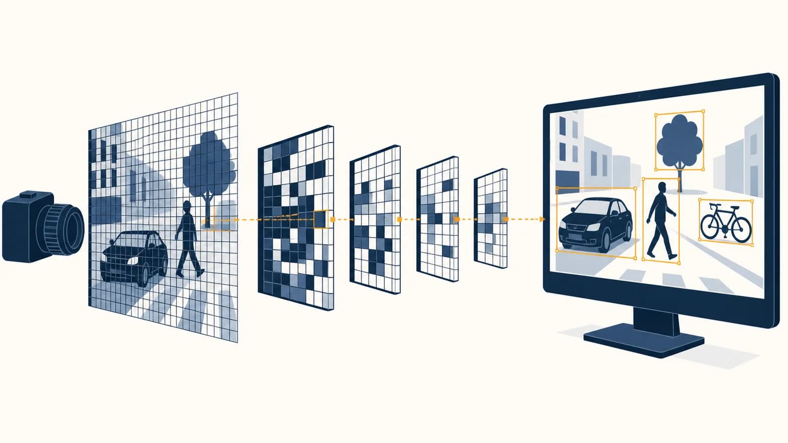
Computer vision is a field of artificial intelligence that extracts useful information from images and video, in the context of computing. A computer vision system turns pixel values into answers such as what an object is, where it appears, how it is moving, or whether a visible defect is present. People searching for how computers see, image recognition, object detection, facial recognition, or AI vision are asking about different parts of this field. The idea exists because cameras collect more visual data than people can inspect quickly and consistently.
A camera does not hand a computer a miniature scene with objects already named. It supplies measurements arranged in a grid. Software must connect patterns in those measurements to a task defined by people. That gap between measured light and useful meaning is the central problem of computer vision.
What a digital image actually is
A digital image is a rectangular array of numerical samples called pixels. Each pixel records light measured at one small location, usually as separate red, green, and blue channel values. The numbers describe color and brightness, not objects or meaning.
Suppose an image is 640 pixels wide and 480 pixels high. It contains pixel locations. If it uses three color channels, the model receives values. A grayscale copy needs one value per location, while a depth camera may add a measurement of distance.
The third card describes a chosen example, not a universal video standard. At 30 images per second, one minute contains frames. A vision program may process every frame, sample some of them, or track changes between frames to reduce work.
Pixel values depend on the camera. A typical image sensor measures incoming light through colored filters, then hardware and software turn those measurements into an image. Exposure, white balance, lens distortion, compression, and sensor noise all affect the final numbers. Two cameras aimed at the same chair can therefore produce different arrays.
Pixels do not contain labels. The number at a location cannot announce that it belongs to a wheel, a face, or a cloud. Meaning comes from patterns across many pixels and from the task used to interpret them.
Programs usually store an image as a tensor, which is a multidimensional array. A color image can have height, width, and channel dimensions. A batch used in training adds another dimension for the number of images. This representation lets processors apply the same arithmetic to many locations at once.
How a computer vision system works
A computer vision system captures an image, converts it into a consistent numerical form, computes informative patterns, produces a task-specific prediction, and checks that prediction against rules or evidence. The exact model changes, but this input-to-decision pipeline remains recognizable.
Consider a conveyor camera checking bottles for missing caps. The camera first captures each bottle at a fixed point. Preprocessing may crop the belt, resize the image, and scale channel values into a numerical range expected by the model. The model then computes features and returns a score for “cap present.” Application code compares that score with a chosen threshold and may signal an air jet to remove the bottle.
Specify the output before choosing a model. “Find every bottle cap” is testable; “understand the factory” is not.
Collect images from the cameras, angles, lighting conditions, products, and unusual cases the deployed system will meet.
Resize, crop, correct distortion, or normalize values in the same way during training and later use.
Run an algorithm that maps the prepared array to a class, location, mask, measurement, or other required output.
Apply thresholds, physical constraints, tracking, or human review before the prediction changes anything outside the program.
Older systems often used hand-written feature rules. An engineer might search for a circular edge in a known region, because a cap viewed from above looks roughly circular. Modern systems often learn useful features from labeled examples. Both approaches can be combined. A learned detector might locate the bottle, while geometric code measures the cap diameter in millimetres after camera calibration.
The difference between a demonstration and a working system often appears after the prediction. A raw score is not yet a safe decision. The surrounding program must handle missing frames, multiple objects, low light, time limits, contradictory sensors, and cases that deserve human inspection. the programming ideas used to turn computations into reliable procedures explain much of this surrounding logic.
What visual features actually are
A visual feature is a numerical pattern that helps distinguish relevant image content. Simple features describe edges, corners, color changes, or texture. Learned features combine such local patterns into increasingly task-specific representations, such as parts, shapes, or object-level evidence.
An edge appears where nearby pixel values change sharply. If a row of grayscale values is 20, 22, 21, 180, 184, the jump between 21 and 180 is evidence of a boundary. It could be an object outline, a stripe, or a shadow. Context decides which interpretation is useful.
A convolution measures a small pattern at many image locations. The program places a small grid of weights over one patch, multiplies matching entries, adds the products, then shifts the grid and repeats. One simplified output value is:
For a 2 by 2 patch and weights , the result is .
The same weights are reused across the image. That makes the operation sensitive to the same pattern wherever it appears. In a convolutional neural network, training adjusts many such weights. Early layers often respond to local changes. Later layers combine earlier outputs across larger areas, so their activations can represent arrangements that matter to the task.
One neuron contains a complete little drawing of a cat, and the network compares the input with that stored drawing.
Many units respond to distributed numerical patterns. Their combined activations support the final cat score, and no single unit needs to hold a complete cat template.
Some vision models divide an image into patches and use attention to relate information across them. Attention calculates how strongly one representation should use information from others. This can connect distant regions, such as the two wheels of a partly hidden bicycle. Convolutions and attention are different computational tools, and many practical systems use ideas from both.
How training turns examples into a model
Training adjusts a model’s numerical parameters so its outputs better match known answers on example images. A loss function measures error, backpropagation assigns portions of that error to parameters, and an optimizer makes repeated small updates that tend to reduce it.
Imagine a classifier with two outputs, “cap present” and “cap missing.” For one training image, the model might assign probabilities 0.35 and 0.65 even though the cap is present. A loss function gives that answer a penalty. Backpropagation uses the chain rule of calculus to calculate how changing each parameter would change the loss. The optimizer moves parameters in directions expected to lower future loss.
If the model gives the correct class probability , the loss is . If it gives , the loss falls to about .
One example cannot teach the full task. The training set needs relevant variation: intact caps, missing caps, different bottle colors, reflections, slight rotations, and normal manufacturing marks. Data augmentation can create controlled changes such as crops, flips, or brightness shifts. An augmentation is useful only if it preserves the correct answer. Flipping a road sign may produce an image that could never occur in the intended setting.
Training accuracy alone does not show that the model learned a reusable pattern. A model can memorize details of the training images. Engineers therefore keep validation data for choosing settings and test data for a final estimate on unseen examples. The split must respect the real source of similarity. Nearly identical frames from one video should not be scattered across training and test sets, because the test would then be easier than deployment.
This process is a specific use of how computers learn statistical mappings from examples. Computer vision supplies image structure, visual tasks, and camera-related problems, while machine learning supplies general methods for fitting and evaluating predictive models.
A label is an instruction, not pure truth. If annotators disagree about where a blurry object begins, the training target contains that uncertainty. Written labeling rules and review matter because the model learns from the recorded answer.
Classification versus detection versus segmentation
Classification assigns a label to an image or region, detection locates separate objects with labels and boxes, and segmentation labels individual pixels. The tasks answer different questions, so a model that succeeds at one does not automatically solve the others.
| Task | Typical output | Question answered | Bottle example |
|---|---|---|---|
| Classification | One or more class scores | What is in this image? | “This image contains a capped bottle.” |
| Object detection | Boxes, labels, and scores | What objects are present, and where? | A box around each bottle and each cap. |
| Semantic segmentation | A class for every pixel | Which pixels belong to each kind of material or object? | Every belt pixel, bottle pixel, and background pixel receives a class. |
| Instance segmentation | A separate pixel mask for each object | Which exact pixels belong to each individual object? | Each overlapping bottle gets its own mask. |
| Pose estimation | Landmarks or joint coordinates | Where are meaningful parts? | Points mark the bottle neck, shoulders, and base. |
The output should match the decision. A wildlife camera that only needs to report whether any fox appeared may use classification. Counting foxes needs detection or instance segmentation. Measuring the area of skin affected by a visible condition calls for segmentation, followed by careful clinical interpretation. Asking for more detailed output usually increases annotation effort and creates more ways to be wrong.
Detection systems commonly compare a predicted box with a labeled box using intersection over union, abbreviated IoU. It divides the overlapping area by the total area covered by either box.
If two boxes overlap over 60 square units and their union covers 100 square units, .
An IoU value describes geometric agreement, not whether the label itself is correct. A box can fit a dog perfectly while the model calls it a cat. Evaluation therefore checks location, class, and confidence together. The threshold for acceptable overlap also belongs in the test definition, because a loose box may be adequate for counting but useless for precise robotic grasping.
Computer vision versus human vision
Human vision is a biological perception system connected to attention, memory, body movement, and broad experience. Computer vision is engineered computation over sensor measurements for a defined output. Similar results do not imply that both systems use the same process or understand alike.
A person can see a partly hidden mug, reach behind a book, and infer how the mug continues out of sight. That judgment uses shape knowledge, physical expectations, depth cues, and the goal of grasping. An image classifier may only map a fixed crop to “mug.” It does not automatically represent the hidden handle, the table’s stability, or what pouring means.
Moves eyes and body, combines several senses, asks for clarification, uses causal knowledge, and can notice that a situation is unfamiliar.
Receives the sensors and inputs engineers provide, calculates its defined outputs, and may remain confidently wrong unless uncertainty checks and operating limits are designed around it.
Computers also have advantages. They can repeat the same numerical test without fatigue, inspect wavelengths a suitable sensor records but human eyes cannot see, and measure tiny coordinate changes precisely. People have different advantages: flexible context, common-sense expectations, and the ability to reformulate a task when the situation changes.
The phrase “the machine sees” is convenient shorthand. It should not hide the mechanism. The machine measures, computes, and outputs. Claims about understanding require separate evidence about what the system can do across unfamiliar conditions.
How computer vision shows up in real settings
Computer vision appears wherever a camera or imaging sensor can turn visible structure into a useful measurement. It supports inspection, navigation, search, scientific analysis, document processing, accessibility tools, and creative software, but each setting demands its own data and error controls.
Factories use vision to inspect and guide
Industrial vision checks whether parts are present, reads printed codes, measures dimensions, and guides robot arms. A controlled station may fix the camera, lighting, distance, and background. That narrow setup is an advantage. If every part arrives in a known pose, simple geometry may outperform a larger learned model and be easier to audit.
A metal part passes beneath a camera. Software first locates two drilled holes, uses their centers to correct for small rotations, and then measures the distance between edges. The system rejects a part only if the calibrated measurement falls outside the manufacturing tolerance. Object detection, geometry, and a business rule each perform a distinct job.
A measurement in pixels becomes a measurement in millimetres only after calibration connects the image to the physical scene. Perspective matters: an object farther from the camera appears smaller. Calibration can estimate camera properties and, for a fixed plane, a mapping between image coordinates and real coordinates.
Vehicles use several sensors to estimate surroundings
Driver-assistance and robotic systems can use cameras to detect lane markings, traffic lights, pedestrians, and other vehicles. Video adds motion clues, but apparent movement can come from the object, the camera, or both. Tracking links observations over time, while depth may come from stereo cameras, motion, or another sensor.
A responsible design does not treat one uncertain image prediction as a complete driving plan. It combines perception with mapping, localization, prediction, motion planning, control, and safety checks. Rain, glare, worn markings, and unusual road layouts test parts of the input distribution that ordinary training images may not cover.
Medicine uses images as evidence, not isolated verdicts
Medical imaging systems can mark regions for review, measure structures, compare scans, or prioritize cases. The image is one part of a clinical decision that may also depend on symptoms, laboratory results, patient history, and additional tests. Performance must be studied on relevant patients, devices, and sites.
A model trained on images from one scanner or hospital may learn processing artifacts correlated with a label. That shortcut can fail elsewhere. Separating data by patient and clinical site, checking different subgroups, and testing prospectively help reveal such problems. High-stakes use also needs a defined response when image quality is poor.
Phones and media tools estimate structure for editing
Phone cameras use vision for focus, exposure, panorama alignment, portrait effects, text capture, and image search. A background blur effect may estimate which pixels belong to the subject, then apply different processing to that mask. Hair, glass, mirrors, and gaps between fingers expose mask errors because their boundaries are visually complicated.
Generative editing and image description often build on representations learned by neural networks that organize many layers of learned features. Their fluent outputs can look persuasive even when a detail was missed, so applications must distinguish visible evidence from generated suggestion.
Four mistakes people make with computer vision
Most mistakes come from confusing a model’s output with direct knowledge of the scene. A score depends on training data, labels, sensors, thresholds, and deployment conditions. Good evaluation tests the whole system against the decision it is meant to support.
1. Treating high accuracy as a complete result
Accuracy is the fraction of tested cases counted as correct. It can hide which errors occurred and how costly they were. In a test set with 90 intact caps and 10 missing caps, a system that always predicts “intact” gets accuracy while finding no missing caps at all.
A confusion matrix separates true positives, false positives, true negatives, and false negatives. Precision asks what fraction of positive predictions were correct. Recall asks what fraction of actual positive cases were found. The useful balance depends on the consequence of a missed defect compared with an unnecessary manual check.
These numbers follow directly from the stated example. They show why one summary metric cannot describe all behavior.
2. Assuming the dataset represents the future
A test set represents deployment only if it includes the conditions that matter. Seasonal light, a replacement camera, new packaging, different skin tones, or a changed road surface can shift the input distribution. Monitoring should look for changes in image quality, input patterns, error rates, and the rate of human overrides.
3. Reading confidence as probability of truth
A model score ranks its own alternatives under learned parameters. It is not automatically a calibrated probability that the statement is true. Calibration tests whether predictions assigned a particular confidence are correct at roughly that rate on suitable held-out data. Calibration can also deteriorate after deployment conditions change.
4. Ignoring the decision around the prediction
The same model can be used safely or badly. A low-confidence match might open a photo folder for the owner, trigger a second sensor, ask a reviewer, or deny someone access. Those actions have different stakes. Thresholds, appeal routes, logging, privacy limits, and human authority belong to the system design.
This sentence is a design rule, not a quotation from a named source. It keeps attention on what happens after the model returns numbers.
How lighting, viewpoint, and occlusion change predictions
Lighting changes recorded brightness and color, viewpoint changes apparent shape and scale, and occlusion removes visible evidence. A model handles these changes only to the extent that its architecture, training data, and surrounding system support the required invariances and missing information.
A white sheet photographed under warm indoor light and blue daylight produces different channel values, even though people still call it white. A plate viewed head-on looks circular, while the same plate viewed at an angle projects as an ellipse. A parked car behind a hedge may expose only its roof and windows. These are changes in measurement, not necessarily changes in the object.
Engineers respond in several ways. They can control the scene with fixed lights and camera mounts. They can augment training images with realistic changes. They can use multiple cameras or depth sensors. They can track an object through video, accumulating evidence over time. They can also define an abstention rule, allowing the system to say that the input is inadequate.
Test the transformation you claim to handle. If a model should recognize a sign at several distances, build a test that changes distance while preserving the sign’s identity. Do not assume that ordinary accuracy proves scale tolerance.
Some transformations should change the answer. Rotating a picture of a screw may preserve its class, but rotating a handwritten 6 can make it resemble a 9. A medically relevant color change should not be normalized away. Invariance is therefore a task choice, not a universal virtue.
How facial recognition differs from face detection
Face detection locates regions that appear to contain faces, while facial recognition compares a detected face with identities or searches for a match. Detection asks “where is a face?” Recognition asks “whose face might this be?” and creates greater privacy risks.
A recognition pipeline often detects a face, aligns landmarks such as the eyes, converts the crop into an embedding vector, and compares that vector with enrolled examples. Similarity does not establish identity by itself. The application chooses a threshold, and that choice trades missed matches against false matches.
Verification and identification are also different. Verification compares a presented face with one claimed identity, such as a device owner. Identification searches a collection for possible identities. Searching more candidates creates more opportunities for misleadingly similar matches, so evaluation must reflect the actual search setting.
A phone may use a face match as one private signal and offer a passcode after failure. A public authority searching video across a large identity database affects people who never chose to participate. Similar vector arithmetic sits inside both systems, but consent, error consequences, data retention, and routes for challenge are very different.
Images of faces are personal data, and biometric templates can be especially sensitive because a person cannot replace their face like a password. Technical questions about matching accuracy sit beside legal and policy questions about collection, purpose, retention, access, and oversight.
How a vision model can be tested before people rely on it
A vision model should be tested on unseen, representative cases with metrics tied to the intended decision, then challenged under important variations and failure conditions. Testing must include the camera, preprocessing, thresholds, timing, and human workflow, not only the model file.
Start with a written claim: “Under the specified inspection lighting, the system flags missing caps for human review.” That sentence identifies the object, condition, output, and decision. A test plan can then include ordinary products, rare cap types, glare, partial views, line stoppages, and images with no bottle present.
Keep test cases independent of training, including independence by person, product batch, location, or video sequence where those links could leak information.
Report error types separately and examine performance for conditions and groups that the deployment claim covers.
Vary brightness, blur, camera position, obstruction, background, and object appearance within realistic limits.
Disconnect a camera, send a corrupt image, create an empty frame, and check that uncertainty produces a safe response.
Log suitable signals, sample cases for review, detect distribution changes, and define who can stop or update the system.
Error analysis is more useful than a single leaderboard number. Group mistakes by cause: small objects, blur, reflections, label ambiguity, background confusion, or preprocessing failure. Then change the data, task, camera setup, or model based on a specific diagnosis. Sound data analysis connects these measurements to defensible conclusions.
Privacy testing also belongs here. A system may be accurate yet collect more imagery than its purpose requires. Designers can ask whether processing can happen on the device, whether faces or license plates can be removed, how long images must be stored, and who can retrieve them. Data minimization can reduce harm before any prediction is made.
The takeaway: Judge a computer vision system by a specific task, representative evidence, visible failure modes, and the consequences of its decisions. A striking demonstration is only the start of that case.
Computer vision makes perception a testable computing problem
Computer vision turns measured light into defined outputs through data structures, algorithms, learned parameters, and evaluation. Its value comes from making a visual task precise enough to compute and test, while keeping the limits of sensors, data, and decisions visible.
The field connects many parts of computing. Images become arrays in memory. Algorithms transform those arrays. Models learn parameters from examples. Programs connect outputs to interfaces and machines. Security protects cameras and stored images. Data analysis checks whether the system works for the cases it claims to handle. You can place those connections within the wider set of computer science ideas and applications.
A useful way to study any vision feature is to trace one prediction all the way through. Name the light source and sensor. Write down the array shape. Identify each preprocessing operation. State the exact output. Ask where the training labels came from. Calculate one metric by hand. Then follow the output into the action it causes.
Try that trace the next time a phone isolates a portrait, a shop scans an item, or a camera reads a road sign. Look for the pixels, the learned or programmed pattern, the threshold, and the consequence. Once those pieces are visible, “the machine saw it” becomes a claim you can inspect.