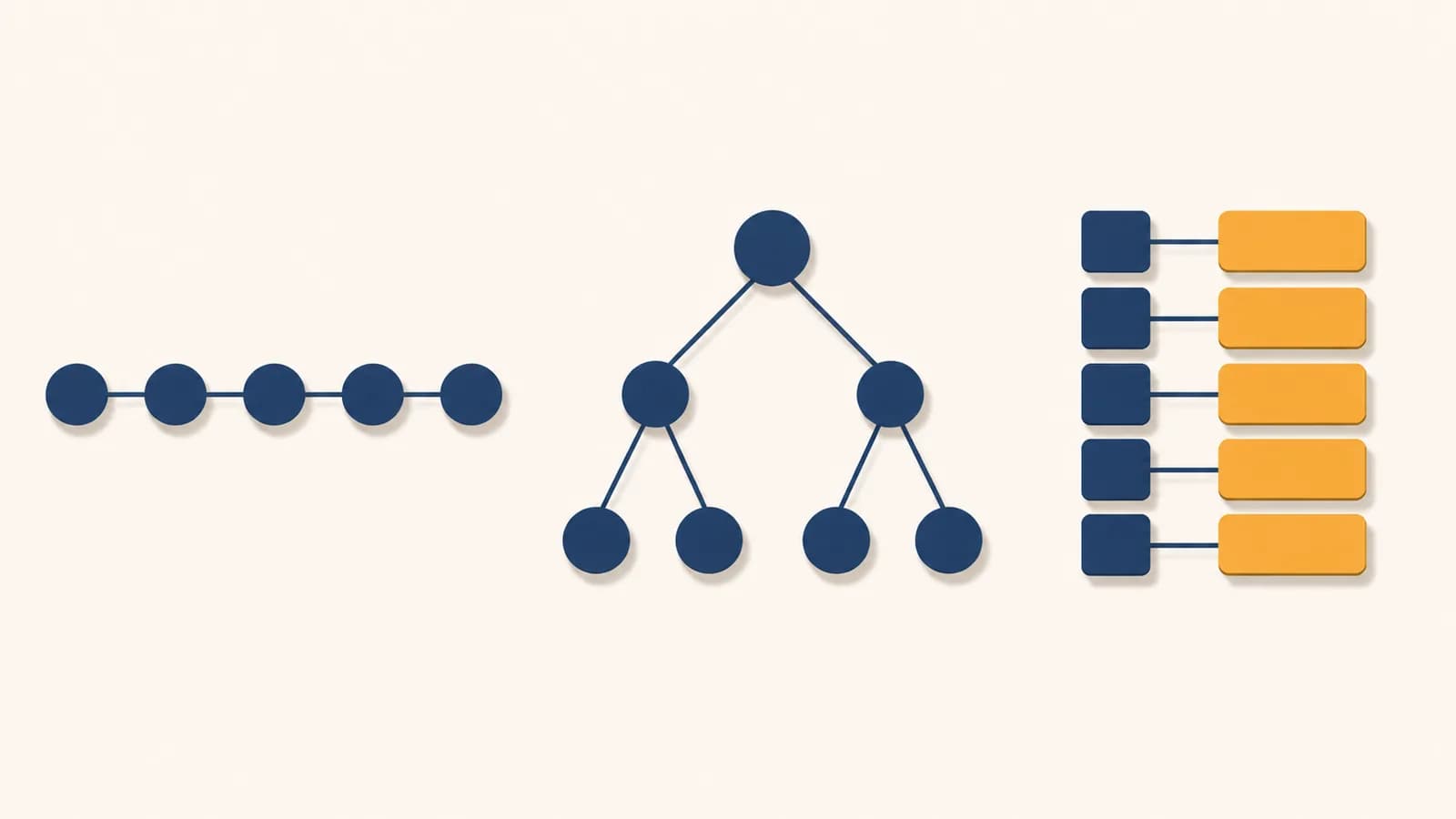
Data structures are organized formats that store and connect data so software can access and change it efficiently, in the context of computer science. Lists, trees, and maps are three common data structures, alongside arrays, linked lists, binary trees, and hash maps. Each gives data a different shape and makes some operations faster or simpler than others. Data structures exist because a computer needs precise rules for finding, inserting, updating, and removing information. A contact list, a folder tree, and a map from usernames to accounts may contain similar pieces of data, but they answer different questions well.
What a data structure actually is
A data structure is a defined arrangement of values plus the operations allowed on them. It specifies which values are connected, how a program reaches them, and what work is required to add, find, change, or remove one.
Consider six student records. The records could sit one after another in an array, each with a numbered position. They could form a linked list in which every record points to the next. They could hang beneath parent nodes in a tree. They could also be stored in a map that uses each student ID as a key. The records have not changed. Their arrangement has, so the useful operations have changed too.
An operation is an action such as reading the item at position 4, looking up the record with key S104, inserting an item, or visiting every item. Computer scientists compare the cost of those operations as the amount of data grows. Big O notation expresses that growth. An operation described as takes a bounded amount of work independent of the collection size in the model being used. An operation may inspect every one of items.
Those labels describe growth, not an exact stopwatch reading. Memory layout, processor caches, language overhead, and the size of each record also affect real speed. A sensible design begins with the questions the program must answer most often, then selects a structure whose operations match those questions. The broader ideas behind variables, references, and loops appear in the foundations of how programs store and process values.
How a list works
A list works by keeping items in a definite sequence, so each item has a position relative to the others. Programs use lists when order, repetition, and iteration matter, such as songs in a queue or steps in a recipe.
Suppose a playlist contains Amber, Blue, Cedar, and Drift. The first item comes before the second, and the list may legally contain Blue twice. A program can visit the songs from beginning to end, insert a new song after Blue, or remove the item at a chosen position. Unlike a map, the list does not require every song to have a unique lookup key.
Many languages implement their everyday list type with a dynamic array. Its elements occupy a continuous run of numbered slots. If the first slot has address and each slot occupies bytes, the address of index follows a simple relation.
If , , and , the slot begins at address .
That calculation explains why reading an array item by index is normally . Inserting at the front is different. Existing elements must shift one place to preserve the sequence, so inserting into an array of items can require moves. Appending is usually cheap while spare capacity remains.
The dynamic array checks whether an unused slot remains after the final item.
If the storage is full, the implementation reserves a larger block and copies or moves the existing items into it.
The program places the value in the next slot and increases the stored length.
A growth operation is expensive, but it does not occur on every append. Implementations commonly reserve extra space when they grow. Spread across many appends, the average cost per append stays constant under the usual amortized analysis. This is called amortized , not a promise that every individual append takes equal time.
Lists versus linked lists
An array based list stores neighboring items in neighboring slots, while a linked list stores each item in a separate node with a reference to another node. Both preserve sequence, but their access and editing costs differ.
Indexing is direct. Iteration tends to use memory efficiently. Inserting near the front may shift many items, and growth may move the entire array.
Reaching index requires following links from a known node. Inserting after a known node changes a few references, but every node stores link information.
Take the linked sequence Amber to Blue to Cedar. To insert Birch after Blue, create a node for Birch, make it point to Cedar, then change Blue so it points to Birch. The other nodes do not move. If the program knows only the head and asks for index 2, however, it must follow the first link and then the second.
A singly linked node points forward. A doubly linked node points both forward and backward, which makes removal and reverse movement easier when the program already has the relevant node. Those extra references use memory. In real systems, dynamic arrays are often faster for ordinary iteration because nearby elements fit processor cache behavior well. Big O describes how work grows, but it does not erase those constant costs.
What a tree actually is
A tree is a collection of nodes connected by parent and child relationships, with one root and no cycles in the standard rooted form. It represents hierarchy and supports searches that repeatedly choose among smaller branches.
A file system presents a familiar tree. A folder can contain files and more folders. Each contained folder can have children of its own. Starting at the root, the path School/Science/notes.txt selects one child at each level. The slash separated path records the choices through the hierarchy.
Tree vocabulary is literal enough to picture but precise enough to code. The root has no parent. A leaf has no children. A node's depth counts edges from the root to that node. The tree's height is the greatest depth, under a common convention. A subtree consists of a node and all its descendants.
A tree has exactly one path from the root to each node. If two distinct routes can lead to the same node, or a route can loop back, the structure is a graph rather than a tree in the strict data structure sense.
A binary tree allows at most two children per node. A binary search tree, or BST, adds an ordering rule: keys in a node's left subtree compare lower, and keys in its right subtree compare higher. The ordering rule, not the two child limit alone, enables directed search. More general network structures and their path finding methods belong to the study of routes and connections in graphs.
How a binary search tree works
A binary search tree works by comparing a target key with the current node, then continuing left for a lower key or right for a higher key. Search ends when the key matches or the required child is empty.
Insert the keys 8, 3, 10, 1, 6, 14, 4, and 7 in that order. The first key, 8, becomes the root. Key 3 goes left because it is lower than 8. Key 10 goes right. To place 4, compare it with 8, then 3, then 6. The decisions are left, right, left, so 4 becomes the left child of 6.
To find 7, compare it with 8. Since 7 is lower, continue to node 3.
Seven is higher than 3, so continue right to node 6.
Seven is higher than 6, so continue right and find node 7.
The work is proportional to the path length, so it depends on height. A balanced BST with nodes has height on the order of . A badly shaped tree can become a chain. Inserting 1, 2, 3, 4, and 5 into a plain BST produces only right children, giving height and linear search in the worst case.
Every binary search tree gives search because each node has no more than two children.
Logarithmic search needs bounded height. Self balancing designs such as AVL trees and red black trees use rotations and stored rules to prevent extreme skew.
Tree traversal visits every node in a chosen order. Inorder traversal of a BST visits the left subtree, the node, then the right subtree, which yields keys in sorted order. Preorder visits a node before its subtrees and can help serialize a hierarchy. Postorder visits children before their parent, a useful order when calculating folder sizes or deleting descendants before their container.
What a map actually is
A map is a data structure that associates each unique key with a value. It answers lookup questions by key, such as finding an account by username, without requiring the caller to know a numbered position.
A map might associate red with #FF0000, green with #00FF00, and blue with #0000FF. The color names are keys, and the codes are values. Assigning a new value to the key red normally replaces its existing value. Two different keys may point to equal values, but a key identifies at most one current value inside a standard map.
Maps are also called dictionaries, associative arrays, or symbol tables in different languages and contexts. The interface usually offers insertion, lookup, update, deletion, and a membership test. The interface does not dictate one implementation. A hash table and a balanced search tree can both implement a map, with different guarantees.
| Question | Useful structure | Reason |
|---|---|---|
| What value belongs to this exact key? | Hash map | Expected constant time lookup with a suitable hash function and controlled load |
| What is the next key after this one? | Ordered tree map | Keys remain in comparison order |
| What item is at position 12? | Array based list | Direct indexed access |
The word map can also mean the operation that applies a function to every item in a collection. That operation and the key value data structure are separate concepts. Context usually resolves the meaning: “put this user in the map” refers to storage, while “map this function over the list” refers to transformation.
How a hash map works
A hash map works by converting a key into an integer hash, reducing that number to a bucket location, and resolving cases where different keys select the same bucket. It then checks keys for equality before returning a value.
Imagine a small table with eight buckets. For a worked example, use the deliberately simple hash rule “sum the character codes,” then choose a bucket with the remainder after division by 8. Real hash functions mix input bits more carefully, but the bucket step has the same shape.
If a key has hash 43, then , so the table begins its lookup at bucket 3.
A collision occurs when distinct keys choose the same bucket. Collisions are normal because possible keys greatly outnumber buckets. In separate chaining, each bucket holds a small collection of entries. In open addressing, the table probes other slots according to a rule until it finds the key or an empty slot. A correct implementation stores the original key and confirms equality, because matching hashes do not prove matching keys.
The load factor compares stored entries with available buckets. For entries and buckets, it is . As a table becomes crowded, collisions and probes tend to increase. Implementations resize the backing table and place entries again using the new bucket count. That resize can be expensive, while ordinary insertion remains expected under standard assumptions about hashing and load control.
Never treat a hash as proof that two values are equal. Hashes are compact fingerprints, so collisions can exist. Compare the actual keys after locating a candidate entry.
A key must behave consistently while stored. If a program inserts a key, then changes the fields used to calculate its hash, a later lookup may search the wrong bucket. Languages often restrict mutable objects as keys or require programmers to define equality and hashing together. Security sensitive tables may also defend against inputs chosen to cause many collisions, since a pileup can turn fast expected behavior into slow linear work.
Lists versus trees versus maps
Lists organize by position, trees organize by parentage or comparison order, and maps organize by unique key. The right choice follows the questions a program asks most, plus any ordering, memory, and worst case guarantees it must preserve.
| Structure | Primary relationship | Strong operation | Typical tradeoff |
|---|---|---|---|
| Array based list | Item before or after item | Read by index, append, sequential scan | Middle insertion may shift items |
| Linked list | Node points to neighboring node | Insert near a known node | Index lookup requires traversal |
| Balanced search tree | Parent, child, and key order | Ordered search, predecessor, range query | More links and balancing work |
| Hash map | Unique key associated with value | Expected fast exact key lookup | No inherent sorted order, collisions need handling |
Suppose an application stores appointments. A list can retain the order in which appointments were created. A balanced tree keyed by start time can efficiently find the next appointment or all appointments within a time interval. A hash map keyed by appointment ID can fetch one exact record quickly. A mature program may maintain all three views and update them together.
A library checkout system keeps each member's current loans in a list, indexes books by catalog ID in a map, and may use an ordered tree for reservations sorted by date. One book record participates in several structures because each structure answers a different operational question.
Choosing a structure also affects algorithms built on top of it. Binary search needs indexed, sorted data. Breadth first traversal needs a queue. Memoization stores previously solved inputs in a map, a technique explained through reusing solutions to smaller computational problems. The data structure is part of the algorithm, not a storage box added after the thinking is finished.
How data structures show up in real software
Data structures appear wherever software must preserve order, represent containment, or retrieve a record by identity. Interfaces, databases, compilers, network services, and games combine them so each frequent operation has a suitable path through the data.
A browser keeps history and page structure differently
A browser can model back and forward history with stack like sequences. Visiting a new page adds an entry. Going back moves through earlier entries, while visiting a fresh page after going back can discard the old forward branch. The document itself is represented as a tree of elements. A paragraph node can contain text and links, while a list node contains item nodes. Changing one subtree lets the browser update the corresponding part of the display.
A compiler uses maps to connect names with meanings
When source code refers to a variable named total, the compiler must determine which declaration that name means. A symbol table maps names to information such as type, scope, and storage location. Nested scopes can be represented by linked tables or a stack of maps. The parsed program is commonly stored as an abstract syntax tree, where an addition node has operand children and a loop node owns its condition and body.
A database builds extra structures for faster questions
A database table stores rows, but scanning every row for every query would waste work. An index builds an additional structure over selected columns. Tree based indexes support ordered ranges such as all orders between two dates. Hash based indexes suit exact matches in systems that provide them. Every index consumes storage and must be updated when indexed data changes, so faster reading can make writing more expensive.
A game tracks space and identity with separate views
A game may keep entities in a list for a frame by frame update loop and a map from entity IDs to entity objects for exact lookup. A spatial tree divides the game world into regions, then subdivides crowded regions. Collision detection can test nearby objects instead of comparing every object with every other object. The visible result is smooth motion, but the hidden work is careful organization.
Data structures also encode policy. A queue serves earlier arrivals first. A priority queue serves the item with the highest or lowest priority according to its rule. A map overwrites or rejects a duplicate key depending on its interface. Those are observable behaviors, so selecting a structure can affect fairness, predictability, and error handling as well as speed.
Four mistakes people make with data structures
Most data structure mistakes come from naming a structure without stating its operations, assuming average performance is guaranteed, ignoring memory behavior, or forcing one structure to answer every query. Each mistake can be corrected by making requirements explicit.
1. Treating a map as automatically ordered
Some language implementations preserve insertion order for their standard map type, while others expose no useful order, and a sorted map uses key order rather than insertion order. Code that depends on iteration order should choose an interface that promises it. An observed order in one run is not a contract.
2. Quoting Big O without naming the operation
Saying “linked lists are ” is incomplete. Inserting after a known node can be constant time. Finding the node at index is linear. Deleting by value may require a scan first. State the operation, the input already available, and whether the claim is worst case, average case, or amortized.
3. Ignoring the shape of real input
A plain binary search tree looks efficient on randomly mixed keys but becomes a chain on sorted insertion. A weak hash function can cluster keys. Test data should include ordered keys, repeated prefixes, duplicate attempts, empty collections, and the largest realistic collection. Adversarial or simply repetitive input exposes assumptions that friendly examples hide.
4. Duplicating data without maintaining consistency
Keeping the same records in a list, tree, and map can speed several queries, but every insertion, update, and deletion must maintain all views. If an update reaches the map but not the tree, later queries disagree. Centralize mutations, use database transactions where appropriate, and test invariants after changes.
Useful invariant: if a map indexes every record in a list by ID, then the map size must equal the number of distinct IDs in the list, and every mapped record must appear in that list.
How do stacks and queues fit?
Stacks and queues are sequence interfaces defined by removal order. A stack removes the most recently added item first, while a queue removes the earliest remaining item first. Arrays or linked nodes can implement either interface.
Undo history often uses a stack: push each completed action, then pop the latest action to reverse it. A print service uses a queue when jobs should run in arrival order. The words describe permitted behavior, not necessarily one memory layout. This distinction between an abstract data type and its implementation lets programmers change storage without changing calling code.
Can one data structure contain another?
Data structures can contain other data structures, and useful software routinely nests them. A map can hold lists as values, a tree node can hold a map of attributes, and a list can store trees representing documents.
Consider a class schedule stored as a map from weekday to a list of lessons. The key Monday finds Monday's list, and index 0 finds its first lesson. Each level answers a different question. Nesting is useful when the access pattern has layers, but deeply nested updates need clear rules for missing keys, empty collections, and shared references.
How do you choose a data structure?
Choose a data structure by listing the required operations, identifying which ones dominate, and selecting the structure whose guarantees fit those operations. Then measure the real program, because data size and memory behavior can change the practical result.
- Name the identity rule. Decide whether items are addressed by index, unique key, parent path, priority, or some combination.
- Name the dominant operations. Count lookups, ordered scans, range queries, front insertions, appends, and deletions.
- Choose the guarantee. Decide if expected performance is acceptable or if the program needs a worst case bound.
- Include storage and maintenance. Account for links, spare capacity, indexes, resizing, and the cost of keeping several views consistent.
- Test representative input. Measure with realistic sizes and patterns, including empty and unfriendly cases.
A small collection often makes clarity more valuable than a theoretical speed difference. A list scan over ten settings may be simpler and fast enough. A service handling a large changing index may need a map or balanced tree. The decision should follow evidence and constraints, not a rule that one named structure is always fastest.
The takeaway: organize data around the questions the program must answer. Use lists for sequence, trees for hierarchy or ordered branching, and maps for key based lookup, then verify the costs that matter.
Data structures turn program behavior into concrete choices
Data structures connect abstract algorithms to memory and observable behavior. They determine the route a program takes to find information, the work required to change it, and the rules users experience when items are ordered, grouped, or retrieved.
The next time an app opens a folder, suggests a contact, restores an undo step, or finds an account, notice the question being answered. Is it asking for a position, a branch, or a key? That question points toward the hidden structure. Comparing those choices is one way to see how data and algorithms fit into computer science as a whole, and it turns performance claims into explanations you can test.