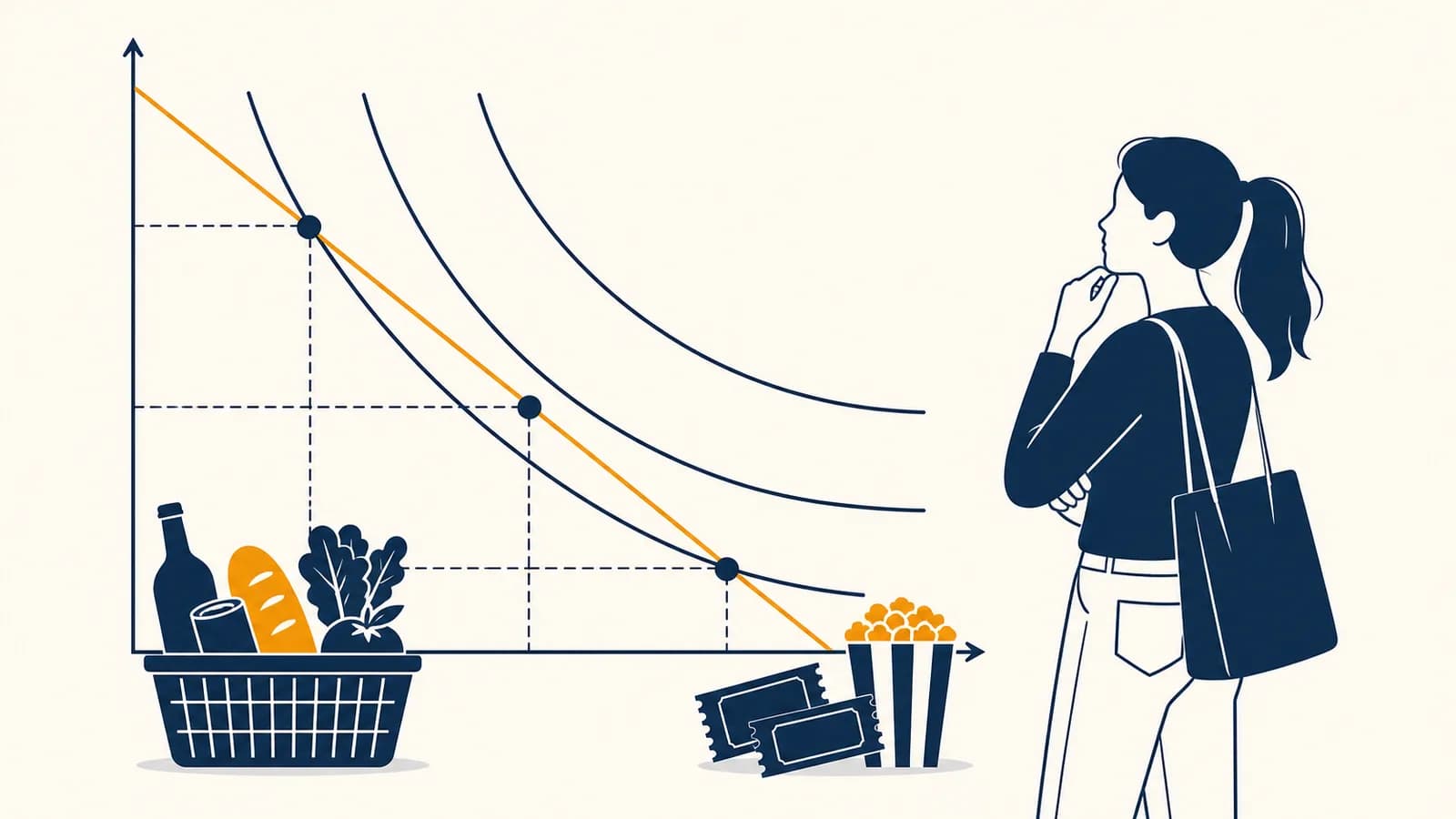
Consumer choice theory is an economic model that explains how people allocate limited income among goods and services, in the context of consumer decision-making. It connects consumer behavior to utility maximization, a budget constraint, indifference curves, marginal utility, prices, and income. The idea exists because every buyer faces scarcity: choosing more of one thing usually means giving up something else. The model does not claim that shoppers solve equations at a checkout. It gives economists a precise way to predict how a change in price, income, or preferences can alter the bundle a person chooses.
Suppose Maya has $60 for lunches and cinema tickets this week. A lunch costs $6 and a ticket costs $12. Her income permits ten lunches, five tickets, or many mixtures between those endpoints. Consumer choice theory asks which affordable mixture she prefers and how her answer changes if ticket prices fall, her budget rises, or her tastes change.
What consumer choice theory actually is
Consumer choice theory represents a buyer using three elements: preferences over possible bundles, a limit set by income and prices, and a choice rule that selects the most preferred affordable bundle. Together, these elements turn scarcity into a testable prediction about demand.
A bundle is a specific quantity of goods or services. Three lunches and two tickets form one bundle. Five lunches and one ticket form another. The model compares complete bundles because real choices interact. Money spent on a ticket cannot also buy lunch.
Preferences rank those bundles. If Maya would choose three lunches and two tickets over five lunches and one ticket when both are free, the first bundle ranks higher for her. Economists often represent that ranking with a utility function. Utility is an index of preference, not a substance stored in a product and not a medical measure of happiness.
The feasible set contains every bundle Maya can afford. Her final choice is the highest-ranked bundle inside that set. This gives the theory its basic logic:
This framework is part of microeconomics, the study of individual buyers, sellers, and markets. It links to the wider set of economics explanations because individual choices combine into market demand, which then interacts with supply to influence prices and quantities.
How the budget constraint works
A budget constraint marks every bundle a consumer can buy at given prices and income. Bundles below the boundary leave money unspent, bundles on it use the entire budget, and bundles beyond it are unaffordable under the model’s stated conditions.
Let be lunches, be cinema tickets, and be their prices, and be the available income. The affordable set is described by:
For $6 lunches, $12 tickets, and $60 of income: .
On the budget line itself, Maya spends all $60, so . If she buys no tickets, she can buy ten lunches. If she buys no lunches, she can buy five tickets. A bundle of six lunches and two tickets costs , so it lies on the line. A bundle of eight lunches and two tickets costs $72, so it lies outside the feasible set.
The line’s slope is . Here it is . The negative sign shows a tradeoff. One additional lunch costs half the price of a ticket, so staying on the same budget requires Maya to give up half a ticket for each extra lunch. With indivisible tickets, only whole-number bundles may be available, but the continuous line remains a useful approximation.
A change in income shifts the line without changing its slope if prices stay fixed. A change in one price rotates the line because one intercept changes while the other does not. That geometry matters: income changes purchasing power across both goods, while a single price change also alters the rate at which the market lets the buyer exchange one good for the other.
How preferences and indifference curves work
Indifference curves join bundles that a consumer ranks equally, so each curve is a contour of preference. Curves farther in the preferred direction represent better bundles, while the curve’s slope shows how much of one good compensates for losing another.
Imagine that Maya values four lunches and two tickets exactly as much as six lunches and one ticket. Those bundles lie on the same indifference curve. She is indifferent between them in the technical sense: if offered either at no cost, her preference ranking gives neither an advantage.
Standard consumer theory usually assumes preferences are complete and transitive. Completeness means Maya can rank any two bundles or regard them as equal. Transitivity means that if she prefers bundle A to B and B to C, she also prefers A to C. Without transitivity, a stable best choice might not exist.
Another common assumption is that more of a desirable good is preferred to less, other quantities held constant. Under that assumption, indifference curves slope downward. If Maya loses a ticket, she needs additional lunches to remain equally satisfied. Curves also cannot cross under consistent preferences. A crossing would make the same bundle belong to two supposedly different preference levels and create a contradiction in the ranking.
Utility numbers are usually ordinal. If one bundle has utility 20 and another has utility 10, the first ranks higher. It does not follow that the first gives exactly twice as much satisfaction.
The slope of an indifference curve is called the marginal rate of substitution, or MRS. Its absolute value tells us how much the consumer is willing to give up for one extra unit of while staying equally well off. For a differentiable utility function, , where each marginal utility measures how utility changes when one quantity increases slightly.
Many textbook preferences produce convex indifference curves. Convexity represents a taste for mixtures and a diminishing MRS. A person with many lunches but few tickets may surrender several lunches for one ticket. After gaining more tickets and losing lunches, the next ticket is less attractive relative to lunch. This is an assumption about preferences, not a universal law. Perfect substitutes can produce straight lines, and goods consumed only together can produce right-angled curves.
How utility maximization works
Utility maximization finds the affordable bundle with the highest preference ranking. For a smooth interior solution, the chosen indifference curve just touches the budget line, making the consumer’s willingness to trade equal to the market’s price tradeoff.
The reasoning can be carried out in a fixed order. It separates what the consumer wants from what the market permits.
Use income and prices to identify every affordable bundle: .
Use stated preferences, an indifference map, or a utility function to determine which bundles rank above others.
Locate the highest indifference curve that still touches the feasible set. Check endpoints as well as any interior tangency.
Confirm that the bundle is affordable and that no available alternative gives higher utility.
For an interior solution with smooth curves, the tangency condition is:
The consumer’s willingness to trade for equals the tradeoff offered by market prices.
Why does equality identify the best interior point? Suppose Maya’s MRS says one more lunch is worth one whole ticket to her, but the market asks her to give up only half a ticket. Lunch delivers more preference value at the margin than it costs. She can improve her bundle by buying more lunch and fewer tickets. That adjustment continues until her personal tradeoff matches the price ratio, unless she reaches an endpoint first.
A tangency is not guaranteed. If Maya regards tickets as extremely valuable relative to lunches at every affordable bundle, the best choice may be five tickets and no lunches. This is a corner solution. Discrete goods create another complication because the exact touching point may be impossible. Then Maya compares the utility of nearby affordable whole-number bundles.
Marginal utility versus total utility
Total utility ranks the whole bundle, while marginal utility measures the added utility associated with one more unit of a good. A choice depends on marginal benefit relative to marginal cost, so the good with the greatest total benefit need not receive the next dollar.
Suppose a person assigns the following utility index to successive slices of pizza during one meal. The numbers are invented preference units for a worked example, not measured facts.
| Slices eaten | Total utility | Marginal utility of latest slice |
|---|---|---|
| 0 | 0 | Not applicable |
| 1 | 20 | 20 |
| 2 | 35 | 15 |
| 3 | 45 | 10 |
| 4 | 50 | 5 |
Total utility keeps rising, but each added slice contributes less than the one before it. That pattern is diminishing marginal utility. It can help explain downward-sloping demand: as a person consumes more, the extra unit tends to be less valuable, so a lower price may be required to make another unit worthwhile.
For choices across several goods, the useful comparison is marginal utility per unit of currency. If another slice adds 10 utility units and costs $5, it provides units per dollar. If a drink adds 6 units and costs $2, it provides units per dollar. Shifting $2 toward the drink can improve the bundle, provided quantities are adjustable and the utility numbers represent the same person’s ranking.
How highly does the consumer rank everything consumed so far?
How much does the ranking index change if one more unit is added?
The equality rule is another form of the tangency condition. If the ratios differ, moving spending toward the good with higher marginal utility per dollar can raise utility. If all relevant ratios are equal and the budget is exhausted, no small reallocation improves the interior bundle.
How price and income changes reshape choices
A price or income change alters the feasible set, which can move the chosen bundle even when preferences stay fixed. A price change creates both a substitution effect and an income effect, while an income change creates only a purchasing-power effect.
Suppose the ticket price falls from $12 to $6 while Maya’s $60 budget and the lunch price remain unchanged. Her maximum number of tickets rises from five to ten. The budget line rotates outward around the ten-lunch intercept. Tickets are now cheaper relative to lunches, and Maya can also afford bundles that were previously beyond reach.
A streaming service cuts its monthly price while other prices and a household’s budget stay fixed. Streaming becomes cheaper relative to cinema visits, which encourages substitution. The lower bill also leaves more purchasing power for all normal goods, including goods unrelated to entertainment.
The substitution effect isolates the response to the new relative price while holding the consumer at the original level of utility. A cheaper good tends to be chosen more because it now costs less in terms of the alternatives surrendered. This effect always moves consumption toward the relatively cheaper good under the standard model.
The income effect captures the change in real purchasing power. A price fall makes the same money budget able to purchase more. For a normal good, greater purchasing power raises quantity demanded. For an inferior good, greater purchasing power lowers quantity demanded because the consumer shifts toward a preferred alternative.
The observed change in quantity is the sum of those two effects. For a normal good, both effects support greater consumption after its price falls. For an inferior good, they oppose each other. The substitution effect usually dominates, so demand still slopes downward. The rare theoretical exception appears when the opposing income effect is larger, producing a Giffen good.
An increase in money income shifts the entire budget line outward in parallel if prices do not change. The response depends on the type of good. The model therefore connects individual choice to how unequal incomes shape the options households can actually afford. Preferences matter, but access to the feasible set matters too.
How consumer choice shows up in shops, jobs, and public policy
Consumer choice theory appears wherever someone predicts demand or designs an offer under limited budgets. Retailers, subscription businesses, transport planners, benefit designers, and policy analysts use its logic to study tradeoffs, responses to price changes, and differences among buyers.
Retailers use demand estimates to decide package sizes, discounts, shelf space, and inventory. A supermarket considering a discount on coffee wants to know how many buyers will switch from tea, how many will buy extra coffee, and how much spending will move from unrelated products. Those are substitution and purchasing-power questions, even if the spreadsheet does not display an indifference curve.
Subscription businesses create menus of bundles. A basic plan, a standard plan, and a premium plan combine features with different prices. Each customer selects from a constrained set. Firms study which features cause a buyer to move between plans and how a price rise affects cancellations. The choice is not simply “buy or do not buy.” It is a ranking across bundles that include quality, advertising, storage, contract length, and money left for other uses.
Employers also confront consumer choice through compensation. A worker may value cash pay, health coverage, retirement contributions, schedule control, and leave differently. A benefit package is a bundle. Tax rules and employer costs create a constraint, while worker preferences determine which package is attractive. The simple theory clarifies the tradeoff even though actual contracts contain uncertainty and legal restrictions.
Governments use the same framework when comparing cash assistance with vouchers or direct provision. Cash expands the recipient’s feasible set broadly. A food voucher expands access to a narrower category and may restrict which bundles can be chosen. The design question is partly about preferences and partly about the public purpose of the program. Broader issues about deprivation and access appear in explanations of how poverty limits development and household choice.
Taxes and subsidies change consumer prices. A tax on a product rotates or shifts the relevant budget boundary inward for that product. A subsidy does the opposite. The private choice calculation still may omit harm or benefit imposed on others. That missing piece is explained by how external costs and benefits sit outside a buyer’s budget. Consumer choice predicts the buyer’s response; welfare economics asks whether the resulting market outcome is socially desirable.
Researchers can also work backward from observed choices. If a buyer selects bundle A when both A and B are affordable, the choice reveals that A ranks at least as high as B under stable conditions. Repeated observations can place restrictions on preferences without asking the buyer to assign numerical utility. This method is powerful, but it requires accurate information about the options, prices, and constraints the person faced.
How real behavior stretches the basic model
The basic model is a benchmark, not a complete account of human behavior. People face limited attention, imperfect information, habits, social pressure, uncertainty, and self-control problems, so an observed purchase may reflect more than stable preferences and a money budget.
A budget has more than one dimension. Money, time, storage, physical energy, and attention can each constrain a decision. A low-priced meal kit may still be unattractive if it requires an hour of preparation. A free app can carry an attention cost. An accessible model should include the constraint that actually binds.
Information is also costly. Comparing every phone contract may take longer than the expected saving is worth. A consumer may use a shortcut, such as choosing a familiar brand or the middle option. This can be sensible under a search cost, even though it differs from the textbook image of a fully informed optimizer.
Choices can depend on presentation. A default option may be accepted because changing it requires effort. A price framed as a small daily amount may feel different from the same amount billed annually. Losses may influence behavior more strongly than equivalent gains. Behavioral economics studies these patterns and builds models that retain constraints and incentives while changing assumptions about judgment and preference.
The consumer has stable preferences, knows the available options, and selects the most preferred affordable bundle.
The consumer may search selectively, follow a default, misjudge future needs, or treat time and attention as additional scarce resources.
These complications do not make the benchmark useless. They show what must be added to explain a particular setting. If a price cut does not increase sales, analysts can check quality beliefs, switching costs, stock limits, social meaning, or delayed consumption. The model supplies a disciplined starting prediction, and deviations help identify missing mechanisms.
Four mistakes people make with consumer choice
Most errors come from treating a simplified model as a moral claim or a literal picture of thought. Consumer choice theory describes constrained rankings under stated assumptions. It does not prove that choices are wise, that utility is measurable happiness, or that markets capture every consequence.
1. Calling every chosen bundle affordable in a broad sense
The formal budget constraint uses the income assigned to the decision and the relevant prices. Real buyers may borrow, draw down savings, receive gifts, or face future bills. A purchase can satisfy today’s cash constraint while creating a harder constraint next month. The analyst must define the time period and resources honestly.
2. Treating utility as pleasure with a physical unit
Utility usually records a ranking. Many different number systems can represent the same ordering. If ranks bundles, a strictly increasing transformation such as preserves that ranking. The transformed numbers change, but the predicted choice does not. This is why claims about one person having “twice the utility” of another usually lack meaning in basic consumer theory.
3. Assuming a tangency must be the answer
The equation applies to a smooth interior optimum. Perfect substitutes often produce an endpoint. Quantity restrictions can create corners. Indivisible goods require comparison among separate points. A solution method that checks only derivatives can miss the actual best feasible bundle.
4. Confusing private choice with social benefit
A buyer can maximize personal utility while imposing noise, pollution, congestion, or another cost on people outside the transaction. The budget line includes prices paid by the buyer, not every cost to society. Policy analysis therefore needs more than consumer choice alone.
Observed choice is not automatic proof of approval. A person may select the least harmful option in a poor feasible set, lack information, face coercion, or choose under an urgent constraint.
How consumer choice explains normal, inferior, and Giffen goods
Normal, inferior, and Giffen goods are classified by how quantity demanded responds to income or price. Normal goods rise with income, inferior goods fall with income, and Giffen goods are inferior goods whose quantity demanded rises when their own price rises.
“Inferior” describes a demand relationship, not product quality. A household might buy fewer instant noodles after income rises because it switches toward meals it prefers. Another household could treat the same noodles as a normal good. Classification depends on the consumer, alternatives, price range, and circumstances.
A Giffen response requires a strong negative income effect that outweighs the substitution effect. Imagine a low-income household relying heavily on a staple because it provides inexpensive calories, with little room in its budget. If the staple’s price rises, the household becomes effectively poorer. It may cut a more desirable food and buy even more of the staple to maintain basic intake. The conditions are demanding, so the category should not be used as a casual explanation for any product whose sales rise with price.
Goods bought partly for status are different. A higher price might make a visible product more desirable because the price itself signals exclusivity. That is commonly discussed as a Veblen effect, which changes the preference or information side of the story. A Giffen effect instead comes from the interaction of substitution and purchasing power for an inferior good.
How choice changes when goods are substitutes or complements
Substitutes can replace each other in consumption, while complements are more valuable when used together. A price change therefore affects demand beyond the product whose price moved: it can redirect spending toward a substitute or reduce demand for a paired good.
Tea and coffee may be substitutes for a particular buyer. If coffee becomes more expensive, the budget tradeoff shifts and tea becomes relatively attractive. The buyer may substitute toward tea. The strength of the response depends on preferences. Someone who dislikes tea has a weak substitute available and may reduce coffee without buying much tea.
Printers and compatible ink are complements because using one raises the value of the other. A fall in printer prices can increase printer purchases and later raise demand for ink. Firms that sell connected products often consider the full system rather than price each item in isolation.
The terms describe relationships, not permanent labels. A bus ride and a bicycle trip may be substitutes for commuting on a dry day, but complements when a cyclist takes a bicycle on public transport for part of a longer trip. The relevant use, location, and time period determine the relationship.
Consumer choice connects scarcity to demand
Consumer choice theory links personal preferences and limited resources to the demand economists observe in markets. Its lasting value is the mechanism: change a price, income, option, or constraint, then trace how the feasible set and best available bundle respond.
The next time a subscription changes its plans or a shop offers a discount, identify the bundle, the constraint, and the nearest alternatives. Ask which part of the choice changed. A lower price may alter both relative cost and purchasing power. A new default may alter attention rather than affordability. A voucher may expand one part of the feasible set while leaving another unchanged.
Those distinctions prevent vague claims about people “wanting more.” They show exactly what the model predicts and where extra evidence is needed. That habit of separating preferences, constraints, incentives, and outside effects is one of the most useful ways to reason about economics.
The takeaway: Consumer choice is the search for the highest-ranked affordable bundle. To analyze a real decision, map the options, prices, income, and other constraints, then check how a change moves the boundary or the ranking.