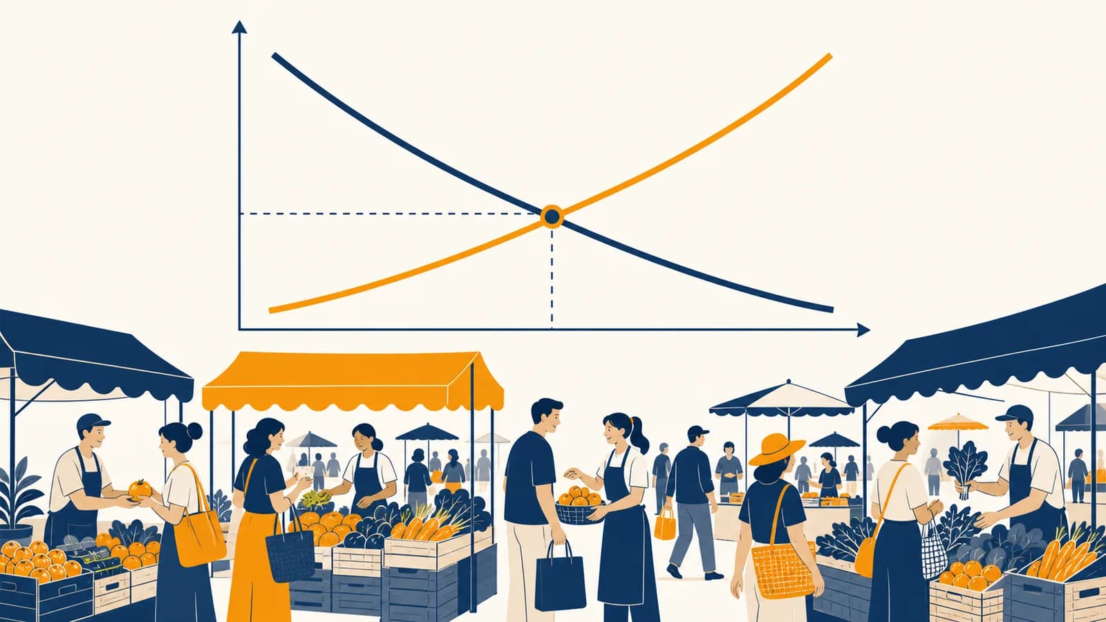
Supply and demand is a market model that explains how buyers and sellers interact to determine prices and quantities, in the context of economics. A supply and demand graph shows how much consumers want to buy and producers want to sell at each possible price. The model exists because scarce goods must somehow be allocated among competing uses. It helps explain why concert tickets become expensive, why strawberries cost less in season, and why some shortages persist even when people are willing to pay.
What demand actually is
Demand is the amount of a good or service that buyers are willing and able to purchase at each possible price during a stated period, with other relevant conditions held constant. It describes a whole relationship between price and quantity, not one purchase.
The words willing and able both matter. Wanting a new laptop does not create market demand unless the buyer can pay for it. Likewise, having enough money does not create demand unless the buyer chooses to spend it on that product.
A demand schedule turns the relationship into numbers. Consider tickets for a small local concert. The quantities below are invented for a worked example, so every result follows from the table rather than from an unsupported claim.
| Ticket price | Quantity demanded | Quantity supplied |
|---|---|---|
| $10 | 900 | 300 |
| $20 | 700 | 500 |
| $30 | 500 | 500 |
| $40 | 300 | 700 |
| $50 | 100 | 900 |
At $20, the quantity demanded is 700 tickets. That is one point on the demand curve. Demand means the full set of price and quantity pairs. Economists usually draw price on the vertical axis and quantity on the horizontal axis. The demand curve slopes downward in this example because a lower price makes the concert affordable or attractive to more buyers.
A demand curve is a conditional statement. It says how much buyers would purchase at each price if income, tastes, expectations, the number of buyers, and prices of related goods did not change.
The downward slope is called the law of demand. It reflects several mechanisms. A lower price lets the same budget buy more. It also makes the item cheaper relative to substitutes. A buyer might choose this concert instead of a movie after the ticket price falls. These mechanisms do not say that every individual behaves identically. They predict the usual direction of the market response.
What supply actually is
Supply is the amount of a good or service that sellers are willing and able to offer at each possible price during a stated period, with other relevant conditions held constant. It is a schedule of possible quantities, not the stock currently sitting on shelves.
In the concert example, a higher ticket price supports a larger supplied quantity. The organizer can rent a larger venue section, hire more staff, or justify adding seats that are costly to manage. At $30, the table says sellers offer 500 tickets. At $50, they offer 900.
The law of supply states that quantity supplied usually rises as price rises, other conditions unchanged. One reason is rising marginal cost. A bakery can make its first loaves with its normal ovens and staff. Producing many more at short notice might require overtime, express ingredient deliveries, or less efficient equipment. Sellers need a higher price before those extra units make sense.
The units a seller already has available, such as 40 bicycles in a warehouse.
The quantities sellers would offer at several prices during a defined period.
Time changes what sellers can do. A café may serve only a few extra lunches today because it has fixed kitchen space. Over a year, it can buy equipment, train workers, or open another location. Supply therefore tends to respond more strongly when producers have more time to adjust.
How market equilibrium works
Market equilibrium occurs at the price where quantity demanded equals quantity supplied. At that price, buyers plan to purchase exactly the amount sellers plan to offer, so neither a shortage nor a surplus creates pressure for the price to move.
In the concert schedule, equilibrium is 500 tickets at $30 each. The arithmetic is visible: quantity demanded is 500 and quantity supplied is also 500. The total amount paid for tickets would be , although that revenue is not the same as profit because the organizer still has costs.
A shortage pushes buyers to compete
A shortage exists when quantity demanded exceeds quantity supplied at the current price. At $20, buyers seek 700 tickets while sellers offer 500, producing a shortage of tickets. Some buyers leave without one.
If price can change, disappointed buyers may bid more, or the seller may notice the fast sales and raise the listed price. As price rises, some buyers drop out and sellers become willing to provide more. The gap narrows. The model predicts pressure on price, not a guaranteed instant adjustment. Contracts, menus, regulation, and concern about customer anger can slow it.
A surplus pushes sellers to compete
A surplus exists when quantity supplied exceeds quantity demanded at the current price. At $40, sellers offer 700 tickets while buyers seek 300, leaving tickets unsold. Sellers then have a reason to cut prices or reduce the number offered.
In the ticket example, both sides equal 500 when the equilibrium price is $30.
Equilibrium is not a claim that everyone is happy or that the outcome is fair. Some people value a ticket but will not pay $30. Some possible seats cost too much to provide at that price. Equilibrium simply means the plans of participating buyers and sellers are mutually consistent at the margin.
How curves move and how movement along a curve works
A price change causes movement along an existing supply or demand curve, while a change in another determinant shifts the entire curve. Keeping these two changes separate is necessary for explaining both the cause and the new market result.
Suppose the concert ticket price falls from $30 to $20 and nothing else changes. Quantity demanded rises from 500 to 700. This is an increase in quantity demanded, shown as movement along the same demand curve. It is not an increase in demand.
Now suppose the performer releases a popular song and more people want to attend at every ticket price. Demand itself increases, so the demand curve shifts right. At $30, buyers might now want 700 tickets instead of 500. The old price then creates a shortage, which puts upward pressure on both equilibrium price and equilibrium quantity.
Specify the product, place, and period. “Coffee” is vague; “cups of takeaway coffee in this town each morning” is workable.
Ask what changed first: the product's own price, buyer income, an input cost, technology, expectations, or something else.
A buyer-side event shifts demand. A seller-side event shifts supply. A change in the product's own price causes movement along both curves.
Compare the old and new intersections. State separately what happens to equilibrium price and equilibrium quantity.
Demand shifts with buyer income, preferences, expectations, the number of buyers, and the prices of substitutes or complements. If bus fares rise, demand for train journeys on the same route may rise because the two are substitutes. If game consoles become cheaper, demand for compatible games may rise because the products are complements.
Supply shifts with input prices, technology, taxes, subsidies, expectations, natural conditions, and the number of sellers. Cheaper flour can increase the supply of bread. A machine that produces each bottle with less labor can also increase supply. An excise tax raises the seller's cost per unit and tends to decrease supply.
Supply and demand versus quantity supplied and quantity demanded
Supply and demand refer to complete relationships between price and planned quantity, while quantity supplied and quantity demanded refer to single amounts at one price. A curve shifts when the relationship changes; a point moves when the product's own price changes.
At every possible price, buyers now plan to buy a different amount. The entire demand curve shifts.
The product's own price changes, so buyers move to another point on the existing demand curve.
The same grammar works on the seller side. A fall in the price of wheat reduces the quantity of wheat supplied, represented by movement down its supply curve. A fall in the price of fertilizer lowers a production cost and increases the supply of wheat, represented by a rightward shift of its supply curve.
This distinction prevents circular explanations. Saying “price rose because demand rose” can be useful if demand means a shifted curve caused by a separate event, such as higher income. Saying “demand rose because price rose” conflicts with the usual law of demand if it refers to movement on one curve. Precise terms reveal which event is cause and which result.
How elasticity measures responsiveness
Elasticity measures how strongly quantity responds to a change in price, income, or another variable. Price elasticity of demand compares the percentage change in quantity demanded with the percentage change in price, allowing responses across different units and products to be compared.
If price rises by 10 percent and quantity demanded falls by 20 percent, elasticity is . Its absolute value is 2.
Demand is called elastic when the absolute value exceeds 1. Quantity changes proportionally more than price. It is inelastic when the absolute value is below 1. Quantity changes proportionally less. The negative sign records the usual opposite movement of price and quantity demanded, while many discussions compare absolute values.
Substitutes make demand more elastic because buyers can switch. Time also matters. A commuter may still buy fuel immediately after a price rise because work and home locations are fixed. Given longer, the commuter can change vehicles, share rides, use transit, or move. A narrowly defined product, such as one brand of cereal, usually has closer substitutes than a broad category such as food.
Elasticity helps a seller anticipate revenue. Revenue equals price times quantity sold. In the computed example above, a 10 percent price increase paired with a 20 percent quantity decrease means quantity responds more strongly. Exact revenue depends on the starting values. If 100 units sell at $10, revenue is $1,000. After those changes, 80 units sell at $11, so revenue is .
Supply has elasticity too. Supply is more responsive when firms have spare capacity, goods can be stored, inputs can be moved between uses, or producers have time to expand. Fresh fish cannot be stored like metal bolts, so sellers face different adjustment limits.
How prices coordinate information and incentives
A market price coordinates separate decisions by carrying information about scarcity and changing the rewards for action. A rising price encourages buyers to conserve or seek substitutes while encouraging sellers to expand output, redirect stock, or enter the market.
Imagine heavy rain damages the local strawberry crop. At the old price, stores have fewer boxes than shoppers want. The shortage gives sellers evidence that the old price no longer balances plans. A higher price does two jobs: it reduces quantity demanded and makes bringing strawberries from farther away more attractive.
A restaurant sees strawberry prices rise. It replaces a strawberry dessert with an apple dessert. A wholesaler pays for refrigerated transport from another region. Neither actor needs a complete report on the crop. The price change alters both decisions.
This coordination can be effective without being morally sufficient. Price allocates goods toward people who are willing and able to pay, which is not the same as allocating them toward people with the greatest need. A wealthy household can outbid a poor household even when the poor household would benefit more. Economics can describe the tradeoff while public policy decides which outcomes society accepts.
Prices also affect where workers and investment go. If demand for electricians grows faster than supply, wages may rise and attract trainees or workers from other fields. Entry takes time because training is not instant. The connection between wages, hiring, and skills is examined in how labor markets match workers with jobs.
How supply and demand show up in daily decisions
Supply and demand appears in everyday prices whenever changing buyer plans meet limited seller capacity. The model can explain seasonal food prices, apartment rents, wages, ride fares, resale tickets, and stockouts, provided the market and time period are defined carefully.
Seasonal food prices reflect two curves
Produce often becomes cheaper during its harvest season because more can reach markets at each price. That is a supply increase. Demand might shift too, perhaps because shoppers prefer the fruit in warm weather. Observing a lower price and larger quantity suggests the supply increase was strong enough to dominate any upward pressure from demand.
Ride fares ration limited cars
After a stadium event, many riders request trips at once. Demand rises while the number of nearby drivers is limited in the short run. A higher fare can persuade some riders to wait, walk, share a trip, or take transit. It can also attract drivers toward the area. The price response changes both sides of the market.
Housing supply changes slowly
If many people move to a city, demand for homes rises. Existing homes cannot multiply quickly, so short-run supply is relatively unresponsive. Prices or rents may rise sharply before construction catches up. Zoning rules, permit delays, building costs, available land, and interest rates can all affect the supply response.
Resale markets reveal changing demand
A ticket's face value records the original sale price, not necessarily the later equilibrium price. If an event becomes more popular after tickets sell out, resale demand may exceed the fixed supply of seats. Resale prices can rise. If interest collapses, sellers may accept less than face value.
The model helps with personal decisions too. Before accepting a high price, identify what moved. Is supply temporarily tight? Are many buyers arriving at the same hour? Can the purchase wait until sellers adjust? A flexible date, substitute product, or different location can move a buyer away from the most competitive part of the market.
How price controls and taxes change the market result
Price controls legally restrict prices, while taxes create a gap between what buyers pay and sellers receive. Both policies change incentives, quantities traded, and who gains or loses, so their effects cannot be judged by looking only at the posted price.
A binding price ceiling creates a shortage
A price ceiling sets a legal maximum. It is binding only if placed below the market equilibrium price. In the ticket example, a ceiling of $20 would hold price below the $30 equilibrium. Buyers demand 700 tickets and sellers supply 500, so the shortage is 200.
The missing price adjustment does not remove competition. Competition can move into queues, waiting lists, personal connections, application rules, or side payments. Some buyers benefit from the lower legal price if they obtain a ticket. Others would willingly pay $30 but receive none.
A binding price floor creates a surplus
A price floor sets a legal minimum. It is binding only if placed above equilibrium. A $40 floor in the ticket example produces quantity supplied of 700 and quantity demanded of 300, a surplus of 400 tickets. If nobody buys the excess, fewer than 700 transactions actually occur.
A tax changes the price on each side
A per-unit tax places a wedge between the buyer's price and the seller's net receipt. If buyers pay $12 and sellers keep $9, the tax is per unit. The quantity traded is generally lower than without the tax because mutually beneficial trades near the old equilibrium no longer cover the tax.
Who sends the payment to the government does not by itself determine who bears the economic burden. The less elastic side of the market changes its quantity less and tends to bear more of the tax through a less favorable price. This is called tax incidence.
Government spending and tax changes can also shift economy-wide demand rather than only one product market. The wider mechanism appears in how fiscal policy affects total spending and output.
5 mistakes people make with supply and demand
Most mistakes with supply and demand come from mixing up curves and quantities, omitting the event that caused a shift, or treating equilibrium as a moral verdict. A correct analysis names the market, the initial change, the affected curve, and the resulting price and quantity.
1. Treating demand as desire
Demand requires both willingness and ability to buy at specific prices. Millions of people may want a beachfront home, but the demand curve records how many can and will purchase at each price. Desire alone does not tell sellers how many transactions can occur.
2. Saying a price rise increases supply
A higher product price usually increases quantity supplied, which is movement along the supply curve. Supply increases only when a nonprice determinant changes, such as lower input costs or improved production technology. The words identify different diagrams and different causal stories.
3. Assuming every price increase comes from demand
Price can rise because demand increases or because supply decreases. The quantity result separates them. Higher demand tends to raise both equilibrium price and quantity. Lower supply tends to raise price but lower quantity. Looking at sales volume can help identify the more plausible cause.
4. Calling equilibrium fair or ideal
Equilibrium describes balance between planned purchases and sales. It says nothing by itself about equal opportunity, need, rights, pollution, or market power. Those questions require additional evidence and standards. A stable market can still impose serious costs on people outside the transaction.
5. Drawing a curve without defining the market
A curve for “transport” mixes bicycles, buses, cars, trains, and flights, each with different buyers and sellers. State the product, geography, and time period. The supply of hotel rooms in one city tonight behaves differently from the supply of hotel stays across a country next year.
Do not infer a curve from price alone. A higher observed price may reflect a demand increase, a supply decrease, or both. Check the direction of quantity and seek evidence about the event that changed conditions.
Real markets add complications. Firms may have power to set prices, buyers may lack information, and a purchase may affect people outside it. Supply and demand remains useful because it gives a disciplined starting point. It does not excuse ignoring the features that violate its simplifying assumptions.
How the model works in unusual cases
Supply and demand can analyze unusual markets if the scarce item, adjustment mechanism, and relevant constraints are stated clearly. Prices may carry only part of the burden, curves can take uncommon shapes, and observed changes can have more than one possible cause.
What happens when both price and quantity change?
Changes in price and quantity together provide clues about which curve shifted. Price and quantity moving in the same direction suggests a demand shift, while movement in opposite directions suggests a supply shift, assuming one main curve moved and other conditions stayed stable.
If both price and sales rise after a favorable product review, an increase in demand fits the evidence. If price rises while sales fall after a factory closes, a decrease in supply fits. These are diagnoses, not automatic proof. Simultaneous changes, measurement errors, inventory adjustments, and delayed responses can produce a more complicated record.
Inflation also needs careful separation from a relative price change. If nearly all prices rise over time, the purchasing power of money is changing. If only coffee becomes expensive because frost damages a crop, coffee has become scarcer relative to other goods. The distinction is developed in how inflation changes the general price level.
Can supply or demand ever slope the other way?
Supply and demand curves usually have their textbook slopes, but unusual incentives can produce exceptions over a limited range. An exception should be explained through buyer or seller behavior rather than treated as proof that ordinary market reasoning has failed.
For labor, a worker offered a higher hourly wage may initially choose to work more because leisure has become more costly. At a sufficiently high income, the worker may instead buy more leisure and work fewer hours. An individual's labor supply curve can then bend backward. That does not imply every labor market supply curve does so.
Some prestige goods may become more attractive to certain buyers because a high price signals status. Even there, quality beliefs, exclusivity, and limited information may be shifting demand rather than reversing an otherwise fixed curve. The analyst must specify what buyers know and what remains constant.
How can a market have no visible price?
A market can allocate a scarce good without a money price by using time, rules, lotteries, status, or administrative decisions. Supply and demand still helps identify scarcity, but the cost paid by users may appear as waiting, effort, uncertainty, or lost alternatives.
A free museum ticket can have a money price of zero and still be scarce. If 1,000 people want 300 timed entries, some other rule must allocate them. First come, first served makes arrival time valuable. A lottery distributes chances. Membership priority favors a defined group. Each mechanism changes who receives access and what behavior people adopt.
A clinic has a fixed number of appointments this week. If patients pay nothing at booking, appointment slots can still carry a time cost through phone queues, forms, travel, or long waits. Zero dollars does not mean zero opportunity cost.
Black markets can appear when legal prices or allocation rules leave strong unmet demand. Their existence does not mean rules are automatically mistaken. It means enforcement costs, access goals, and unintended incentives belong in the policy analysis.
Supply and demand is a way to test a causal story
Supply and demand turns a vague claim about prices into a testable account of behavior. Name the market, identify the first event, shift the correct curve, and check whether the predicted directions of price and quantity match what can actually be observed.
The model connects individual choices to economics as a whole. Scarcity creates tradeoffs. Opportunity cost shapes what buyers and sellers give up. Marginal thinking explains why the next unit may be treated differently from the previous one. Institutions determine which exchanges are permitted and which costs fall outside the market. Those connections continue across the broader set of economics explanations.
Try the method the next time a familiar price changes. Define the exact product and period. Look for evidence about buyers, production costs, available capacity, policy, and substitutes. Then predict quantity as well as price. If the observed pattern disagrees, revise the story instead of forcing the facts into the graph.
The takeaway: Supply and demand explains how planned buying and selling become a market price and quantity. Its value lies in separating causes from results, then checking those results against evidence.