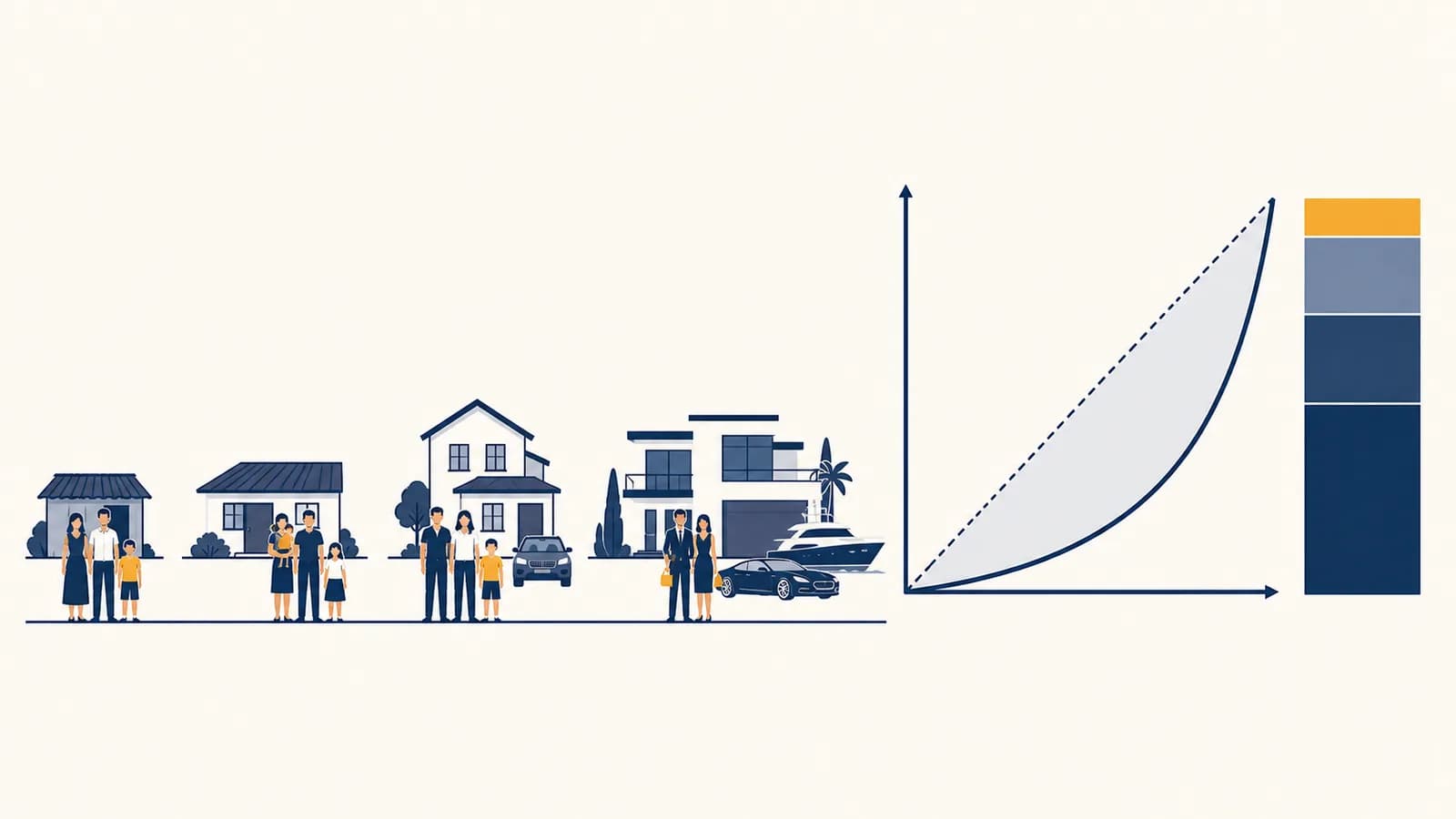
Income distribution is a pattern that shows how total income is divided among people or households, in the context of an economy. Income inequality describes how uneven that pattern is. Economists compare wages, household income, market income, disposable income, and income shares to see who receives what. The idea exists because production creates income, but markets, ownership, taxes, and public benefits do not divide it equally. A distribution can change even when average income stays the same, so the average alone cannot show how living standards are spread.
What income distribution actually is
Income distribution is the full arrangement of incomes across a population, while income inequality is the degree of distance between those incomes. A distribution records both position and spread: who is near the bottom, middle, or top, and how far apart they are.
Suppose five households receive yearly incomes of $20,000, $30,000, $40,000, $50,000, and $60,000. Their total income is $200,000 and their mean income is $40,000. Each household's income share is its income divided by $200,000. The lowest household receives 10 percent of the total; the highest receives 30 percent.
Now change the incomes to $10,000, $20,000, $30,000, $40,000, and $100,000. Total and mean income remain $200,000 and $40,000. Yet the median falls to $30,000, and the highest household now receives half of all income. The economy has the same average income but a more unequal distribution.
An average is not a distribution. Two countries, towns, or workplaces can have the same mean income while giving people very different typical incomes and very different gaps between the top and bottom.
The unit being measured matters. Individual wages describe pay from work. Household income combines resources received by people living together. Household measures often adjust for household size because $60,000 supports one adult differently from a family of five. Analysts must also choose a time period, usually a year, and decide whether to count cash only or include benefits supplied in kind.
How market income becomes disposable income
Market income becomes disposable income when government adds cash transfers and subtracts direct taxes. This sequence separates what people receive through work and ownership from what they can spend or save after pensions, benefits, income taxes, and similar payments are counted.
Labor income includes wages, salaries, bonuses, and earnings from self-employment. Capital income includes rent, interest, dividends, and profits distributed to owners. Together with some private transfers, these form market income. Government retirement payments, unemployment support, and cash assistance can then be added. Personal income tax and required social contributions can be subtracted.
A household with $48,000 of market income, $6,000 in transfers, and $8,000 in direct taxes has $46,000 of disposable income.
This calculation does not automatically include every way government affects living standards. A publicly funded school, hospital, or road provides value without putting cash into a bank account. Sales taxes reduce purchasing power when money is spent, but a basic disposable-income measure may omit them. Housing costs also vary sharply by place. For those reasons, researchers name the income concept they use instead of treating the word income as self-explanatory.
Two parents compare job offers with the same salary. One job includes health insurance and a pension contribution; the other requires the worker to buy both. Their cash wages match, but their compensation and usable household resources do not. Distribution data based only on wages will miss part of that difference.
Prices complete the picture. Nominal income is measured in current money. Real income adjusts for changes in what money buys. If a worker's pay rises by 4 percent while the prices of the goods that worker buys rise by 6 percent, purchasing power falls. A study across years therefore needs a consistent price adjustment. A study across regions may also need to account for differences in rent, transport, and other local costs.
How economists measure inequality
Economists measure inequality by arranging people from lowest to highest income and then summarizing the gaps. Income shares, percentile ratios, Lorenz curves, and the Gini coefficient reveal different features, so a careful comparison uses a measure suited to the question.
Specify individuals or households, the geographic area, the year, and market or disposable income.
Adjust for household size, inflation, and any other differences required by the question.
Order the units from lowest income to highest income, then identify percentiles or equal-sized groups.
Find shares, ratios, or a summary index, then state exactly what a higher or lower result means.
A quintile is one fifth of the ranked population. If 100 households are sorted by income, the bottom quintile is the lowest 20 households and the top quintile is the highest 20. A quintile share asks what fraction of all income goes to each group. Percentiles allow narrower comparisons. The 90th percentile is the income level at or above which the top tenth begins; the 10th percentile marks the corresponding boundary near the bottom.
These bars come directly from the first worked example: $50,000 plus $60,000 is $110,000, which is 55 percent of $200,000. The bar lengths make concentration visible, but the group labels and calculation make the result checkable.
A Lorenz curve plots the cumulative share of people on the horizontal axis against their cumulative share of income on the vertical axis. Perfect equality would follow a 45-degree line: the lowest 20 percent would receive 20 percent of income, the lowest 50 percent would receive 50 percent, and so on. An actual curve usually bows below that line. A deeper bow indicates more concentration.
The Gini coefficient converts the area between the equality line and the Lorenz curve into a number. Zero represents perfect equality. One represents the limiting case in which one unit receives all income and everyone else receives none. Published values may instead appear on a 0 to 100 scale. A Gini value summarizes the whole distribution, but it cannot say by itself where the gaps occur.
Income inequality versus wealth inequality
Income inequality concerns flows of money received over a period, while wealth inequality concerns stocks of assets minus debts at a point in time. A person can have high income but little wealth, or low current income and substantial wealth.
Wages, profits, rent, interest, and transfers received during a month or year. Income is a flow, like water entering a tank.
Homes, savings, pensions, shares, and business assets, minus mortgages and other debts, measured on a date. Wealth is the amount in the tank.
A new doctor may earn a high salary but have negative net wealth because of education debt. A retired homeowner may report modest yearly income while owning a debt-free house and substantial pension assets. Neither case is contradictory. Income and wealth answer different questions about command over resources.
The two distributions interact. Wealth can generate income through rent, dividends, and interest. High income can create wealth when part of it is saved. Wealth can also finance education, a home purchase, or a business, which may raise later income. Inheritance transfers assets across generations without being a wage. These feedbacks help explain why a temporary wage difference and a lasting economic advantage are not the same thing.
Assets worth $260,000 and debts of $210,000 produce net wealth of $50,000.
Consumption offers a third lens. A student may have low measured income while a family pays the student's housing costs. A self-employed person may have uneven yearly earnings but smooth spending with savings. Data on income, wealth, and consumption can therefore tell different but compatible stories.
How labor markets shape the distribution
Labor markets shape income distribution by setting pay through worker productivity, skill scarcity, bargaining power, hours, institutions, and employer demand. Since work supplies much household income, changes in wages or access to paid hours can move the entire distribution.
Demand for a kind of labor rises when employers expect that workers to add more revenue or reduce more cost. Supply depends on how many people can and will do the job, including the time and money needed for training. The interaction resembles the price mechanism explained through how supply and demand set prices and quantities, but a labor contract also involves working conditions, information, law, and bargaining.
Consider two occupations. Training for one takes several years and only a small number of people hold the required license. Training for the other takes a few days and many applicants can perform the tasks. If employer demand is strong in both cases, the scarcer qualification may command higher pay. This is not a moral ranking of the workers. It is a description of how scarcity and demand can affect a wage.
Productivity matters, but it is not a complete pay formula. A worker may produce more because the employer supplies better machinery, software, organization, or access to customers. A large firm may also have more power to set wages when workers have few nearby alternatives. Unions, minimum-wage law, professional licensing, discrimination, contract work, and executive pay rules can all change the link between output and individual compensation.
A warehouse raises its hourly pay after another large employer opens nearby. The workers did not suddenly become more skilled. Their outside options improved, so the original employer had to offer more to recruit and retain staff. A change in competition altered bargaining conditions.
Market structure matters on the product side too. A firm with limited competition may earn persistent profits that can go to owners, executives, workers, or some mixture. The guide to how concentrated markets affect prices and output explains where those profits can come from. Who finally receives them is a distribution question.
Education can raise skills and access to occupations, yet its return varies. The result depends on the field studied, completion, job demand, tuition cost, and the income given up while studying. That forgone income is an opportunity cost because choosing education closes off paid work during the same hours. Treating every qualification as an automatic income increase ignores both cost and labor-market conditions.
How taxes and transfers change the distribution
Taxes and transfers change income distribution by moving purchasing power between households and across stages of life. The result depends on who pays, who receives, how behavior responds, and which public services are counted, not simply on a tax rate's name.
A tax is progressive when the average tax rate rises with the tax base, such as income. It is proportional when that average rate stays constant. It is regressive when the average rate falls as the base rises. These terms describe the share paid, not the number of dollars paid.
A household paying $6,000 of tax on $50,000 of income has an average tax rate of 12 percent.
The marginal tax rate applies to the next unit of taxable income. It is not normally applied to every dollar already earned. Suppose the first $20,000 is untaxed and income above that level is taxed at 20 percent. Someone earning $30,000 pays 20 percent of $10,000, or $2,000. The person's marginal rate is 20 percent, but the average rate is $2,000 divided by $30,000, about 6.7 percent.
Do not multiply total income by the top bracket. In a bracketed system, each rate applies only to income inside its bracket. Moving into a higher bracket does not make earlier dollars face the new rate.
Transfers can target low income, disability, unemployment, children, old age, or other conditions. A benefit may shrink as earnings rise. Its withdrawal then acts like an additional marginal charge because one more dollar of wages produces less than one extra dollar of disposable income. Good analysis combines taxes and lost benefits when estimating the reward from extra work.
Taxes can also change behavior before revenue is distributed. A tax on investment returns may affect saving choices. A payroll tax can influence labor costs and wages. A sales tax changes the price buyers pay and the amount sellers keep. The side legally required to send money to the government is not always the side bearing the full economic burden.
How inequality shows up in daily decisions
Inequality shows up in daily decisions through unequal budgets, risks, time horizons, and access to credit. The same price increase or emergency can produce different choices because households begin with different income, savings, debts, job security, and unavoidable costs.
A household with spare income can buy a durable appliance that costs less to run, pay an annual insurance premium at a discount, or move closer to work. A household with no cash buffer may use a costly short-term loan or keep an inefficient appliance. The second household may understand the long-run saving perfectly but lack the money required today.
A reliable used car costs $8,000. Buyer A pays cash. Buyer B needs a loan and pays interest, plus fees, because work cannot be reached by bus. The sticker price matches, but the cost of obtaining transport does not. Income and wealth affect the available choice set.
Housing creates similar effects. Rent may consume a larger income share for a low-paid household even if that household rents a smaller home. A deposit requirement can block a move that would reduce commuting costs. A homeowner may gain wealth when local property values rise, while a renter in the same area faces a possible rent increase. One market event can change groups' positions in opposite directions.
Firms meet the distribution in their customer base. A grocery store chooses product sizes and price points partly from local budgets. A bank evaluates income stability and collateral when making loans. A government deciding how to fund street lighting or flood control faces the financing problems described in how public goods create shared benefits. Distribution affects both who can pay and who gains protection.
Inequality also appears at work. Employees with savings can search longer after leaving a poor job. Workers supporting dependants may prefer predictable hours over a higher but uncertain hourly rate. Someone with family money may accept an unpaid internship that another equally capable person cannot afford. These are economic constraints, not evidence that one person values success more.
4 mistakes people make with income inequality
Four common mistakes are treating inequality as poverty, reading correlation as cause, ignoring the measurement unit, and assuming every change is a fixed-pie transfer. Each error can turn a correct statistic into a false claim about people's lives or policy effects.
1. Inequality and poverty are treated as the same condition
Poverty is insufficient resources relative to a defined standard; inequality is unevenness across the entire distribution. A society can reduce poverty while inequality rises if low incomes grow but top incomes grow faster. It can reduce inequality during a severe recession if top incomes fall sharply while low incomes do not improve.
Do people have enough resources to meet a specified absolute or relative threshold?
How far apart are incomes, and what share of total income does each part of the population receive?
Both questions matter, but they require different evidence. A poverty rate needs a threshold and a count below it. An inequality measure uses relationships among incomes across much or all of the population.
2. A relationship is presented as a proven cause
A correlation between inequality and another outcome does not identify the direction or mechanism of causation. Inequality might affect health, political power, or growth. Those outcomes might also affect inequality, or a third factor might influence both.
For example, a technological change could raise demand for certain skills and increase wage gaps. The same change might increase total output. A simple observation that inequality and output rose together cannot show that inequality caused the output increase. Researchers look for timing, comparison groups, natural experiments, or other evidence that separates competing explanations.
3. The population and income definition are ignored
An inequality number has no clear meaning until the population, unit, period, and income concept are named. Individual earnings among full-time workers will differ from disposable household income among all residents. Neither is automatically wrong.
Students, retirees, unemployed adults, and people working part time may disappear from a full-time wage study. Household data can hide unequal control of money inside a household. Annual data can make a temporarily unemployed worker look very different from data averaged across several years. Before comparing two numbers, check that their definitions match.
4. The economy is assumed to be a fixed pie
A distribution can change because shares change, total income changes, or both change together. One group's gain does not mechanically equal another group's loss, although bargaining, market power, taxes, and ownership can transfer income between groups.
Return to the five-household example. If every income doubles, the shares and common relative inequality measures remain unchanged, while every household has more nominal income. If only the lowest income rises, inequality falls and total income rises. If the highest income rises while all others stay fixed, total income and inequality both rise. Growth and distribution are separate dimensions that must be checked together.
How mobility changes the picture
Income mobility is movement through the distribution over time, and it changes how a snapshot should be interpreted. High mobility can mean temporary low income, but it does not erase current hardship or guarantee that people from different families face equal chances.
Intragenerational mobility follows the same person across adulthood. A trainee may move upward after qualifying; a worker may move downward after illness or job loss. Intergenerational mobility compares outcomes between parents and children. It asks how strongly family circumstances predict later income, education, or occupation.
Relative and absolute mobility differ. A person's real income can rise while that person's rank stays the same because other incomes rose too. That is absolute progress without relative movement. Another person can rise from the fourth decile to the sixth while real income barely changes during a stagnant period. That is relative movement without much improvement in purchasing power.
Panel data, which follows the same people, is needed to observe movement directly. Comparing two separate yearly surveys can show that the distribution changed, but not who moved. The low-income group in the second survey may contain different people from the low-income group in the first.
How much inequality can a society accept?
No economic formula identifies one universally acceptable level of inequality. The judgment depends on causes, consequences, mobility, poverty, rights, and social values. Economics can estimate tradeoffs and policy effects, while the acceptable distribution remains partly an ethical and political choice.
Some income differences can reward training, effort, risk, innovation, or unpleasant work. They can help direct workers and investment toward uses that buyers value. Other differences may reflect inherited advantage, discrimination, fraud, political privilege, weak competition, or unequal access to education. The size of a gap cannot reveal its source.
Policy choices also have several effects at once. A transfer may raise a family's current resources and improve a child's later opportunities. Its financing may alter work, saving, prices, or business decisions. A tax rule may reduce measured disposable-income inequality but create avoidance opportunities for people able to reorganize their income. Sound evaluation counts the intended distributional change, administrative cost, behavior, and effects on production.
A useful policy debate therefore names the objective. Is the aim to raise the lowest incomes, compress the gap between the middle and top, reduce childhood disadvantage, insure people against shocks, or increase mobility? A policy can succeed on one aim and fail on another. Clear objectives make disagreement easier to test.
Income distribution connects individual choices to the whole economy
Income distribution connects wages, ownership, prices, taxes, public services, and household choices. It shows who receives the value an economy produces and who can command goods and opportunities, so it belongs beside growth, inflation, employment, and efficiency in economic analysis.
When you encounter a claim about inequality, identify the income concept, population, time period, price adjustment, and measure. Then ask what mechanism could have produced the result. A rise in the top share might come from higher business profits, changing executive compensation, lower incomes elsewhere, or a mixture. The statistic locates a pattern; the mechanism explains it.
The same habit improves everyday decisions. A headline about average pay should prompt a check of the median and the range. A tax proposal should prompt separate calculations for marginal rates, average rates, and benefit withdrawals. A job offer should be evaluated through total compensation, costs, security, and the alternatives it closes.
The takeaway: Read every distribution as a map of who receives what, then trace the routes that created it. Use income shares and inequality measures to describe the pattern, but use labor markets, ownership, institutions, taxes, and transfers to explain it.
This method also shows how income distribution fits into the wider study of economic choices. Notice the next time one average is used to describe a whole population. Ask what the average conceals, which households moved, and what changed in the rules or markets underneath it.