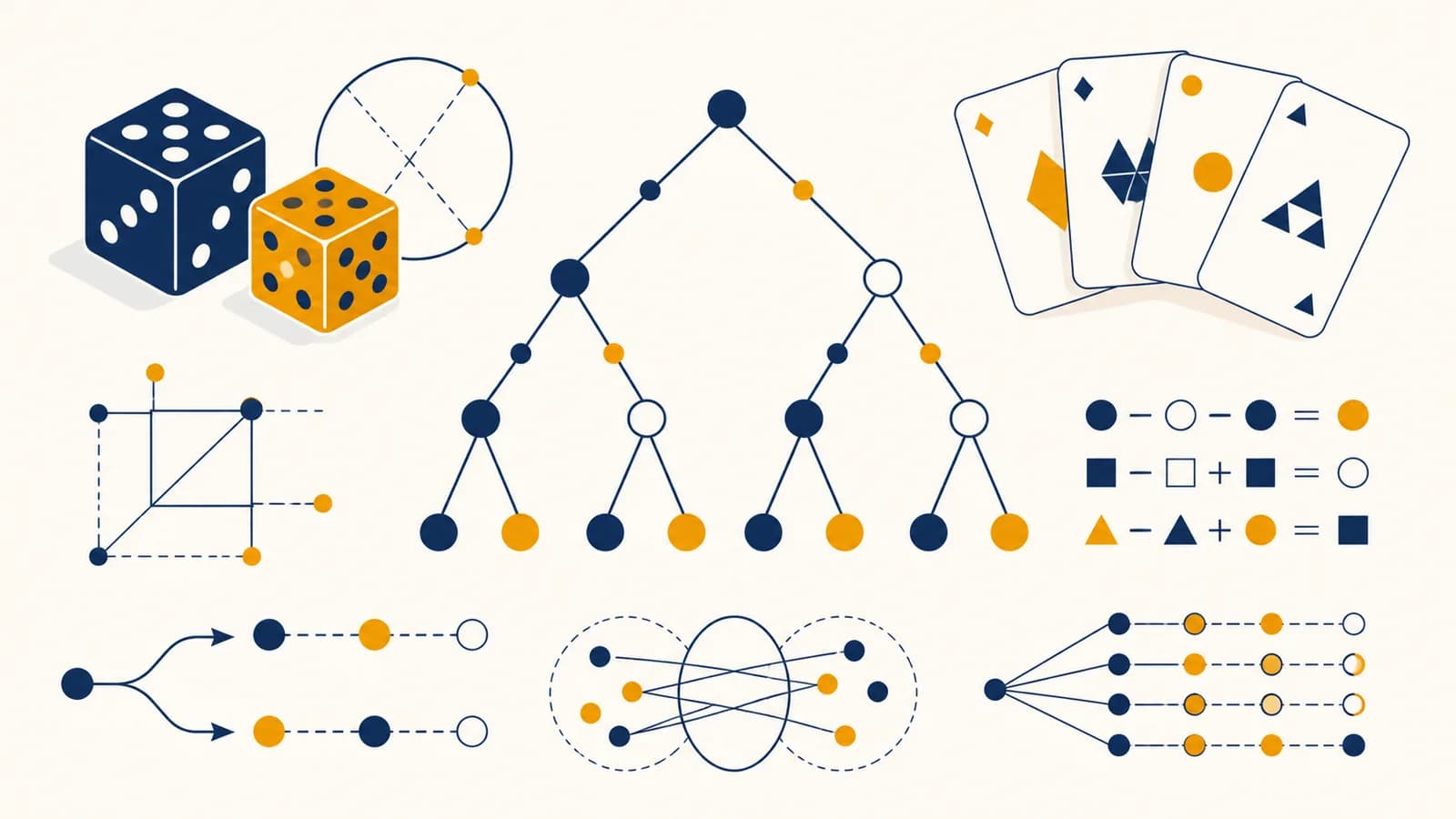
Probability and combinatorics is a branch of mathematics that counts possible outcomes and measures how likely they are, in the context of uncertainty and discrete choices. Probability answers questions such as “What are the chances?” while combinatorics answers “How many arrangements or selections are possible?” The subject includes probability rules, permutations and combinations, conditional probability, independence, expected value, and probability distributions. It exists because decisions often must be made before the result is known, and careful counting turns uncertainty into quantities that can be compared.
A six sided die makes the connection visible. There are six equally likely outcomes, so the chance of rolling a 4 is one out of six. If two dice are rolled, there are 36 ordered pairs, not 12 outcomes. Counting those pairs shows why a total of 7 is more likely than a total of 2: six pairs produce 7, while only one pair produces 2.
Counting comes before probability. If outcomes are equally likely, the probability of an event is its number of favorable outcomes divided by the total number of possible outcomes.
What probability actually is
Probability is a number between zero and one that represents how strongly a model expects an event to occur. Zero means impossible within the model, one means certain, and values between them compare degrees of uncertainty under stated assumptions.
An experiment is a repeatable process with an uncertain result, such as drawing a card. An outcome is one result, such as drawing the queen of hearts. The sample space is the set of all possible outcomes. An event is any selected group of those outcomes, such as drawing any queen.
For equally likely outcomes, the basic ratio is:
A standard deck has 4 queens among 52 cards, so .
The ratio works only if the listed outcomes really are equally likely. The six faces of a fair die fit that assumption. The categories “rain” and “no rain” do not become equally likely merely because there are two of them. A weather model needs observations and physical information, not a count of category names.
Probabilities can also be reported as fractions, decimals, or percentages. A probability of equals 0.25 and 25 percent. The conversion tools in calculating and interpreting percentages help when probabilities must be communicated as rates.
What combinatorics actually is
Combinatorics is the mathematics of counting arrangements, selections, and structures without listing every case one by one. It supplies the denominator and numerator for many probability calculations, especially when a process contains several choices or when order may matter.
The first tool is the addition principle. If one choice can happen in ways and a separate alternative can happen in ways, there are ways to choose one alternative. A cafe offering 5 teas or 3 coffees offers 8 drink choices.
The multiplication principle applies to successive choices. If one stage has options and each can be followed by options, the complete process has outcomes. Four shirts and three pairs of trousers make 12 outfits, assuming every shirt can be paired with every pair of trousers.
A tree diagram expresses the same principle by drawing a branch for each choice. It is useful when later choices depend on earlier ones. For a four digit security code, with ten choices for every position and repetition allowed, multiplication gives possible codes. The ideas behind repeated multiplication appear more generally in working with powers and exponential growth.
How permutations and combinations work
Permutations count selections in which order matters, while combinations count selections in which order does not matter. Both begin with factorials, but combinations divide out the repeated orderings that describe the same selected group.
A factorial multiplies the positive integers down to one:
Five distinct books can be placed in a row in orders.
To arrange objects selected from distinct objects, the first position has choices, the next has , and so on. This produces the permutation formula . Choosing a president, vice president, and secretary from 8 people gives , because changing the assigned offices changes the result.
To choose a committee of 3 from the same 8 people, order is irrelevant. Each group of 3 was counted times by the permutation calculation, once for every internal ordering. Dividing by 6 leaves 56 committees.
For a committee, .
Repeated objects require another correction. The letters in LEVEL have apparent arrangements, but swapping the two Ls changes nothing, and swapping the two Es changes nothing. Therefore the number of distinct arrangements is .
A podium with gold, silver, and bronze positions uses a permutation. The same three runners in different positions produce a different result.
A three person jury uses a combination. Listing A, B, C instead of C, A, B does not create a new jury.
How probability rules combine events
Probability rules combine events by tracking overlap, alternatives, and sequences. The complement rule handles “not,” the addition rule handles “or,” and the multiplication rule handles “and,” with adjustments when events overlap or affect one another.
The complement rule handles everything outside an event
The complement of event , written , contains every outcome where does not occur. Since an event and its complement fill the sample space without overlapping, .
This is especially efficient for “at least one” questions. With three independent coin tosses, the chance of at least one head is easier to find by subtracting the all tails case. The probability of all tails is , so the probability of at least one head is .
The addition rule corrects for overlap
The probability of or is . The overlap is subtracted because it was included once in each of the first two terms.
Draw one card from a standard 52 card deck. There are 13 hearts and 4 kings, but the king of hearts belongs to both groups. Therefore . If two events cannot occur together, they are mutually exclusive, their overlap is zero, and their probabilities can simply be added.
The multiplication rule follows a sequence
The probability that and then occur is . The second factor is the probability of after learning that happened.
Suppose two cards are drawn without replacement. The probability that both are aces is . After the first ace is removed, only 3 aces and 51 total cards remain. Multiplying would ignore that change.
Translate words such as “at least,” “either,” and “both” into a set of outcomes.
Ask if the events can occur together and if learning one result changes the probability of the other.
Use a complement for the opposite event, addition for alternatives, and multiplication for a sequence.
A probability must fall between zero and one, and it should fit the scale of the situation.
How conditional probability changes the sample space
Conditional probability is the probability of an event after some information is known. The condition restricts the sample space, so both the relevant favorable outcomes and the relevant total outcomes must be counted inside the reduced set.
The notation means the probability of given . Its formula is:
Among the 12 face cards in a standard deck, 4 are kings, so .
The condition comes after the vertical bar. Reversing it usually changes the question. Every king is a face card, so , but only one third of face cards are kings. In diagnosis, the difference is the same as distinguishing “the chance of a positive test given illness” from “the chance of illness given a positive test.” Those are not interchangeable.
A two way table can keep the reference group visible. Imagine 100 manufactured parts, classified by production line and inspection result:
| Production line | Pass | Fail | Total |
|---|---|---|---|
| Line A | 54 | 6 | 60 |
| Line B | 32 | 8 | 40 |
| Total | 86 | 14 | 100 |
Given that a part failed, the relevant column contains 14 parts. Of those, 8 came from Line B, so . Given that a part came from Line B, the relevant row contains 40 parts, of which 8 failed, so . The same cell appears in both ratios, but the denominators answer different conditions.
Independence versus mutually exclusive events
Independent events do not change each other’s probabilities, while mutually exclusive events cannot occur together. These ideas describe different relationships and, except for events with probability zero, events cannot be both independent and mutually exclusive.
Two fair coin tosses are independent. Knowing that the first toss is heads does not change the second toss, which still has probability of heads. Thus for the events “first is heads” and “second is heads.”
On one die roll, “roll a 2” and “roll a 5” are mutually exclusive. Once a 2 occurs, a 5 on that same roll is impossible. Their intersection has probability zero. They are not independent because learning that one occurred changes the probability of the other from to zero.
One event gives no information about the other. Test with or .
The events share no outcomes. Test with . Their probabilities add when finding the chance that either occurs.
Replacement often determines independence in sampling. If a marble is drawn, recorded, and returned to a bag before the next draw, the contents reset and the draws are independent. Without replacement, the first draw changes the bag, so the probabilities on later draws change.
Independent does not mean equally likely. A biased coin can produce independent tosses even if heads has probability 0.7 on each toss. Independence concerns influence between events, not fairness.
How random variables and expected value work
A random variable assigns a numerical value to each outcome, and expected value is its probability weighted long-run average. Expected value compares uncertain choices, but it need not be a result that occurs on any single trial.
For a discrete random variable with possible values , multiply each value by its probability and add:
A game paying £10 with probability and £0 otherwise has expected payout .
If entry to that game costs £3, the expected net value is per play. This does not predict a loss of exactly 50 pence on the next play. The only single-play net results are a £7 gain or a £3 loss. The expected value describes the average net result over many repetitions under the same probabilities.
A probability distribution lists the values a random variable can take and assigns probabilities totaling one. Its spread also matters. Two options can have the same expected value but different risks. A guaranteed £5 and a coin toss paying £10 for heads and £0 for tails both have expected value £5, but only one fixes the immediate result.
An insurer cannot know which particular home will make a claim next year. It can estimate a distribution of losses across many policies, combine expected claims with operating costs and uncertainty, and set premiums for the pool. The calculation works across repeated exposures, not as a prophecy for one home.
Expected value is also used in inventory decisions, project planning, medical choices, and quality control. It is a starting summary, not a complete decision rule. A decision maker may also care about worst cases, available cash, fairness, and how uncertain the estimated probabilities are.
How probability shows up in evidence and decisions
Probability turns incomplete evidence into measured uncertainty in fields such as medicine, law, finance, engineering, and forecasting. The calculation is useful only when the model, data source, assumptions, and meaning of the reported probability are kept visible.
Medical tests update an earlier probability
A test result changes a prior probability rather than creating certainty. Suppose 1 in 100 people in a particular screened group has a condition. Imagine a test that returns positive for 90 of 100 people with the condition and also for 5 of 100 people without it. These are hypothetical values chosen to show the arithmetic.
In a modeled group of 10,000 people, 100 have the condition and about 90 of them test positive. Of the 9,900 without it, about 495 also test positive. There are therefore about 585 positive results, with 90 coming from people who have the condition. Under these assumptions, the conditional probability of the condition after a positive result is , or about 15.4 percent.
The example explains why sensitivity alone cannot answer “What is the chance I have the condition after a positive result?” The starting frequency and false positive rate also matter. Actual medical interpretation needs values validated for the relevant test and population.
Courts must separate two reversed conditions
The probability of evidence given innocence is not the probability of innocence given the evidence. Reversing those conditions can make evidence sound far stronger than it is. A rare match may still occur among many possible people, and other explanations for the evidence must remain in the comparison.
Probability does not decide guilt. It can clarify the weight of statistical evidence, but legal judgment also depends on evidence quality, admissibility, alternative accounts, and the required standard of proof.
Engineering uses failure combinations
Reliability calculations track how component failures combine. If a system fails only when two independent backup components both fail, and each has failure probability over the specified period and conditions, the modeled joint probability is . If either single failure stops the system, the structure is different and the risk is higher.
Real components may share a power source, environment, design flaw, or maintenance error. Those common causes break the independence assumption. Engineers therefore use fault trees, testing, and domain evidence instead of multiplying convenient numbers without checking the mechanism.
Forecasts follow the same discipline. A 30 percent rain forecast does not mean rain will fall for 30 percent of the day. Its exact operational meaning depends on the forecasting service, location, time window, and event definition. Good use starts by reading what outcome the percentage describes.
How combinatorics shows up in computing and genetics
Combinatorics appears wherever a finite system can be assembled in many ways. Computing uses it to size search spaces and count codes, while genetics uses it to track possible allele combinations and inheritance patterns under explicit biological assumptions.
Security depends on the size and shape of a search space
A password made of 8 independently chosen lowercase English letters has possible strings. That arithmetic is exact for the stated rule. It does not by itself measure real password security, because people do not choose uniformly at random and attackers exploit common words, reused passwords, leaked data, and system specific limits.
Length changes the count by a multiplication factor. Adding one independently random lowercase letter multiplies the search space by 26. Adding character types changes the factor only if those characters are genuinely used in an unpredictable way. Combinatorics sizes the theoretical space; a threat model explains which parts of that space an attacker must actually search.
Algorithms face combinations too large to list
A route planner visiting locations may need to consider many possible orders. Fixing a starting location still leaves orders in a simple version of the problem. For 11 locations, that is orders. Larger instances quickly make complete enumeration expensive, so algorithms use structure, bounds, approximation, or dynamic programming to avoid testing every order.
Inheritance probabilities come from possible gametes
In a simplified single gene model, two parents with genotype can each contribute or . The four equally likely pairings are , , , and . Grouping the middle two as the same genotype gives probabilities , , and .
This basic counting model assumes equal transmission and ignores factors such as linked genes, selection, new mutation, and complicated traits influenced by many genes and environments. The model is useful because its assumptions are simple enough to test and extend.
5 mistakes people make with probability
Most probability errors come from defining the event poorly, counting unequal outcomes as if they were equal, or applying a correct rule under false assumptions. A reliable solution names the sample space, tests dependence, and checks what the condition actually says.
1. Treating every listed category as equally likely
Two possible labels do not imply a fifty fifty chance. A sports team can win or lose, but that fact alone says nothing about the relative likelihoods. Equal probability must come from symmetry, a randomizing process, or evidence.
2. Adding probabilities when events overlap
Adding and counts their intersection twice. The heart or king example needs one copy of the king of hearts removed. Draw a Venn diagram or list the overlapping outcomes before using the addition rule.
3. Multiplying as though events were independent
Sampling without replacement changes what remains. Shared causes can also connect events that look separate. Use unless independence is justified by the process or supported by evidence.
4. Confusing a run with a correction
After five heads from a fair coin, tails is not “due.” The next toss still has probability of tails if tosses are independent. Long-run balance does not require short sequences to alternate or compensate.
5. Reporting precision the model cannot support
A calculation may produce many decimal places even when its inputs are rough estimates. Extra digits do not repair uncertain data or unrealistic assumptions. State the event, time period, population, and meaningful level of precision. Algebraic expressions can help preserve assumptions before numbers are substituted.
The takeaway: Write the outcomes before reaching for a formula. Most errors become visible once the sample space, event, and dependence between stages are stated in ordinary words.
How can probability be estimated from data?
Experimental probability estimates an event’s chance by dividing its observed frequency by the number of trials. As relevant, well controlled trials accumulate, the relative frequency often settles near the process probability, though any finite sample still contains random variation.
If a machine produces 18 flawed items in 600 inspected items, the observed flaw rate is . That is an estimate for the process under the sampled conditions. It is not proof that exactly 3 percent of every future batch will be flawed.
Sample design matters. Inspecting only items produced during one shift may miss variation across operators, materials, temperatures, or maintenance cycles. A larger biased sample can be less informative than a smaller representative one. The arithmetic of the fraction, covered in interpreting fractions and decimal values, is simple; deciding what the numerator and denominator represent is the harder part.
What is the binomial model?
The binomial model gives the probability of a fixed number of successes in a fixed number of independent trials, when every trial has two outcomes and the same success probability. It combines a probability for each sequence with a count of matching sequences.
For trials, success probability , and exactly successes, the model is:
For exactly 3 heads in 5 fair tosses, .
The combination counts the positions in which the three heads can appear. Every particular five toss sequence with three heads and two tails has probability . Multiplying gives .
The model fails if the trial count is not fixed, outcomes have more than two relevant categories, success probabilities change, or trials influence one another. Drawing from a small deck without replacement, for example, does not keep the same success probability. A binomial formula should follow a check of assumptions, not replace it.
Why can rare events still happen?
A rare event has a small probability on one opportunity, but repeated opportunities can make at least one occurrence much more likely. The correct calculation uses the complement: find the chance that the event never happens, then subtract that result from one.
If an event has independent probability on each of occasions, then:
If across 20 independent opportunities, the chance of at least one occurrence is .
This explains why coincidences become less surprising in a large set of people, dates, transactions, or experiments. Someone who notices a striking result after checking many possible patterns must account for all the opportunities to find something striking. Otherwise the reported probability describes a test chosen in advance, while the actual search examined many tests.
The same logic supports quality control. A tiny defect probability per component may create a meaningful system risk when a product contains many components or when many products are shipped. Independence still needs checking, since one production fault can affect a whole batch.
Probability makes uncertainty part of mathematics
Probability and combinatorics extend mathematics from known quantities to structured uncertainty. Counting defines the possible cases, probability assigns their weights, and evidence updates those weights. Together they make uncertain claims open to calculation, criticism, and revision.
The subject connects arithmetic, sets, functions, algebra, and data. It also teaches a broader mathematical habit: define the object before operating on it. “There is a 20 percent chance” is incomplete until the event, conditions, time period, and source of the number are known. You can place that habit beside the wider set of mathematics ideas and applications.
Try it on the next probability claim you encounter. Write down the event, the relevant sample space, and what information is already known. Ask if the outcomes are equally likely, if events overlap, and if one stage changes the next. Then count. A short calculation may answer the question, and a failed assumption may reveal that the advertised number never answered it at all.