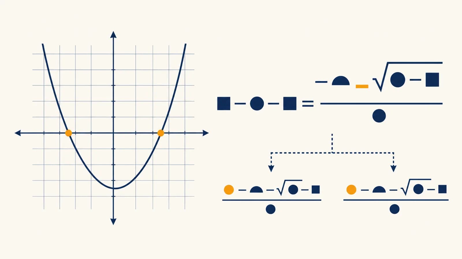
A quadratic equation is an algebraic equation that finds unknown values when the highest power of the variable is two, in the context of mathematics and models of curved change. It has the standard form , where . Solving quadratic equations means finding their roots, also called solutions or zeros. The quadratic formula, factoring, completing the square, and graphing all solve the same basic problem. The idea exists because many quantities do not change at a constant rate: falling objects, areas, distances, and revenue can produce squared terms and therefore quadratic equations.
What a quadratic equation actually is
A quadratic equation is a statement that sets a second-degree expression equal to another expression, usually zero. Its defining feature is a nonzero squared term, and its solutions are the variable values that make both sides of the statement equal.
The word quadratic comes from the idea of a square. In , the variable is multiplied by itself. A quadratic can contain a squared term, a first-power term, and a constant:
In , the coefficients are , , and .
The restriction matters. If , the squared term disappears and the equation becomes linear. The order of the terms does not determine the type. For example, is quadratic because rearranging it gives .
A solution is a value that makes the equation true. For , both and work. Substitution checks them: and . A quadratic equation can have two distinct real solutions, one repeated real solution, or two complex solutions.
Degree controls the maximum number of roots. A quadratic has degree two, so it has at most two distinct real roots and exactly two complex roots when repeated roots and multiplicity are counted.
The equation does not have to begin in standard form. , , and are all quadratic equations. Their forms expose different information, which is why changing form is a central solving skill.
How the parts of a quadratic work
The coefficients , , and control the shape and position of the related parabola. Together they also determine the roots, so reading the coefficients tells you which methods and checks are likely to be useful.
Connect the equation to the function . Solving the equation asks where the graph has height zero. Those locations are the graph's horizontal-axis intercepts. This connection turns an algebra problem into a geometric one.
If is positive, the parabola opens upward and has a minimum. If is negative, it opens downward and has a maximum. The constant is the value of when . The axis of symmetry is , and the vertex lies on that line.
Consider . Its axis is . Substitution gives , so the vertex is . Factoring gives , so the roots are and . Their midpoint is , exactly on the axis of symmetry.
This chain also works backward. If a graph crosses the horizontal axis at and , its quadratic expression contains factors and . An additional nonzero multiplier may change the graph's height without changing those roots.
How the main solving methods work
The main solving methods preserve the same equation while exposing a useful structure. Factoring creates a zero product, completing the square isolates a squared expression, and the quadratic formula packages the general completing-the-square process into one dependable rule.
How solving by factoring works
Factoring solves a quadratic by rewriting it as a product and using the zero-product property. If two factors multiply to zero, at least one factor must equal zero, so each factor creates a smaller equation that can be solved directly.
Start with . Find two numbers whose product is and whose sum is . The numbers are and , so the expression factors as . The zero-product property gives or , hence or .
Rearrange until the equation has the form . The zero-product property depends on the product equalling zero.
Take out any common factor first, then factor the remaining quadratic if possible.
Solve each resulting linear equation. A repeated factor gives a repeated root.
Substitute every candidate solution, especially if earlier algebra involved fractions or rearrangement.
A leading coefficient other than one requires more care. For , split the middle term using numbers with product and sum . Those numbers are and :
The solutions are and . The fraction work here rests on the same operations explained in the guide to reliable basic arithmetic.
Factoring is fast when integer or simple rational factors exist. It is not a universal shortcut. The equation has real roots, but it does not factor into integer binomials. Completing the square or using the quadratic formula handles it cleanly.
How completing the square works
Completing the square turns a quadratic expression into a perfect square plus or minus a constant. This exposes the squared quantity directly, allowing inverse operations to isolate the variable and revealing the vertex of the related parabola at the same time.
For a coefficient of one, take half the coefficient of , then square it. Solve by first moving the constant:
Add the same amount to both sides. Adding only to the left would change the equation. An equation stays balanced only when the same operation is applied to both sides.
The plus-or-minus sign is essential because both and equal . The connection between squares and square roots is developed further in the explanation of roots and radicals.
If the leading coefficient is not one, divide by it first or factor it from the variable terms. For , divide by to get . Move the constant and add :
Completing the square also converts standard form to vertex form. In general, can be written as , where is the vertex. This is useful when the maximum or minimum matters more than the roots.
How the quadratic formula works
The quadratic formula gives every solution of any quadratic equation in standard form. It comes from completing the square on the general equation, and it works even when factoring is awkward or when the solutions are irrational or complex.
For , substitute , , and .
Substitution gives . The expression under the radical is , so . The two results are and . Substitution confirms both.
The formula is easier to remember when its structure is understood. The center of the two roots is , the same as the axis of symmetry. The term measures how far each root sits from that center.
A calculator can evaluate the formula, but it cannot identify the coefficients reliably for you. Put the equation in standard form first, keep the sign attached to each coefficient, and place the whole numerator over . Parentheses prevent most substitution errors.
Quadratic equations versus quadratic functions
A quadratic equation asks for particular values that make an equality true, while a quadratic function assigns an output to every allowed input. They often use the same expression, but one is a problem to solve and the other describes an entire relationship.
asks which inputs make the expression zero. Its answers are and .
assigns an output to each input. Its graph is a parabola with roots and .
The distinction matters in applications. A height function might describe an object's height at every time. Setting that function equal to zero creates an equation whose solutions are the times when the object reaches ground level. The function supplies the model; the equation answers a specific question about it.
A graph can estimate solutions, especially when exact algebra is unnecessary. Yet a drawn crossing is limited by scale and plotting accuracy. Algebra can give exact roots such as , while a graph shows their location and makes unreasonable answers easier to spot.
Do not confuse a quadratic with an exponential expression. In , the variable is the base and the exponent is fixed. In , the base is fixed and the variable is the exponent. Their solving tools differ, and how logarithms reverse exponentials explains the second case.
How quadratic equations show up in motion
Quadratic equations appear in motion whenever position depends on time squared, as it does under constant acceleration. A height model can be set equal to a target height, turning a physical event such as landing into a solvable quadratic equation.
Near Earth's surface, a common simplified model for vertical motion in metres is . Here is initial height and is initial upward velocity. The coefficient is one half of the textbook approximation for gravitational acceleration. The model ignores air resistance and small changes in gravity.
A ball is released from a platform metres above the ground with no initial vertical velocity. The model is . Ground contact occurs when .
Set . Dividing by gives , so and . Algebra gives two roots, but the context removes because it represents a time before release. The ball reaches the ground seconds after release in this simplified model.
This is a general lesson about mathematical models: a valid algebraic root is not automatically a valid physical answer. Units, time direction, measurement limits, and the assumptions behind the formula all constrain the interpretation.
Horizontal and vertical motion can also be combined to describe a projectile path. If horizontal speed is treated as constant, eliminating time often produces height as a quadratic function of horizontal distance. The resulting parabola is an ideal model, not a claim that every real flight path is perfectly parabolic.
How quadratic equations show up in design and money
Quadratic equations arise in design and money when two changing quantities are multiplied or when one change affects both price and sales. The model can locate break-even points, required dimensions, or a maximum, provided its assumptions match the situation.
Suppose a rectangular garden has an area of , and its length is metres greater than its width. If the width is , the length is . The area condition is , or . Factoring gives . The roots are and , but a physical width cannot be negative. The garden is metres wide and metres long.
The same structure appears when a fixed total is split between two factors. A product such as length times width, unit margin times number sold, or speed times a changing travel time can produce a squared term after one quantity is written in terms of the other.
A school club sells tickets at each. For a planning exercise, it assumes each price increase reduces sales by tickets. If is the number of one-dollar increases, modeled revenue is .
Expanding gives . Since , the parabola opens downward, so its vertex represents the model's maximum. The axis formula gives . The model therefore predicts a price of , sales of tickets, and revenue of . Every number follows from the stated assumption, not from observed customer data.
Real demand may not fall in a straight line. Customers may react differently near certain prices, and capacity may impose another limit. A quadratic answer is only as credible as the model that produced it. The algebra can optimize the assumed relationship; it cannot certify the assumption.
Five mistakes people make with quadratic equations
Most errors with quadratic equations come from lost signs, incomplete operations, or answers detached from context. A reliable solution keeps the equation balanced, preserves both square-root branches, checks candidate roots, and states which mathematical answers fit the original situation.
1. Using the zero-product property before one side is zero
The zero-product property applies to a product equal to zero. From , you cannot conclude that either factor is zero. Expand or rearrange first: , then .
2. Losing the second square root
If , then and . Writing only the positive root discards a valid solution. The symbol names the principal nonnegative square root, but solving an equation requires considering both numbers whose square is .
3. Detaching a negative sign from a coefficient
In , the coefficient is , not . Therefore in the quadratic formula. Writing the coefficients with their signs before substituting makes the calculation easier to audit.
4. Dividing by an expression that could be zero
In , dividing both sides by produces , but it silently removes the solution . Factoring and applying the zero-product property preserves both cases.
5. Reporting every root without interpreting it
A negative length is not a usable dimension, and a time before an experiment begins may not answer the question asked. Keep the algebraic root visible, then explain why the domain accepts or rejects it. Context filters results; it does not alter the algebra.
A quick check catches many errors. Substitute each proposed root into the original equation. If the two sides differ, the value is not a solution, regardless of how convincing the intermediate work looks.
Checking also reveals rounding trouble. If an exact radical is available, keep it through the calculation and round only the final measurement. Early rounding can shift a later result enough to matter in a design or timing problem.
What the discriminant actually tells you
The discriminant is the expression inside the quadratic formula. Its sign tells how many real roots a quadratic has because it determines whether the formula takes the square root of a positive number, zero, or a negative number.
| Discriminant | Roots | Graph |
|---|---|---|
| Two distinct real roots | Crosses the horizontal axis twice | |
| One repeated real root | Touches the horizontal axis at the vertex | |
| Two complex roots | Does not meet the horizontal axis |
For , the discriminant is . The expression factors as , so is a repeated root. The parabola touches the axis at and turns around there.
For , the discriminant is . There are no real roots, but the equation still has solutions in the complex numbers: , where .
The discriminant answers the question of root type before you finish solving. It does not by itself give the root values. It is especially useful for checking a graph or deciding whether a proposed physical crossing can occur within a quadratic model.
How you choose the best solving method
The best method is the one that matches the equation's visible structure and the information needed. Square-root methods suit an isolated square, factoring suits simple products, completing the square exposes a vertex, and the quadratic formula handles every standard-form quadratic.
- Use square roots for equations such as .
- Use factoring for equations such as , where the factors are easy to identify.
- Use completing the square when vertex form is useful or the process itself is being studied.
- Use the quadratic formula when factors are not obvious, coefficients are awkward, or a guaranteed general method is preferable.
- Use a graph for a visual estimate, for checking, or when a model is based on measured data and exact roots are not expected.
Method choice affects effort, not truth. For , factoring quickly gives and . The quadratic formula gives the same results after more arithmetic. Completing the square also works, producing .
Keep fractions and radicals, such as . Exact form preserves all information and supports later symbolic work.
Round at the end to a precision justified by the measurements. Include units and state any domain restriction.
If two methods seem equally short, choose the one you can check most clearly. Written structure matters. Good algebra leaves a trail in which signs, operations, and rejected roots can be inspected.
Can every quadratic equation be solved exactly?
Every quadratic equation with known numerical coefficients can be solved exactly within the complex numbers by the quadratic formula. The result may contain fractions, radicals, or the imaginary unit, and a practical problem may still require a rounded or restricted answer.
Some quadratics have rational roots, as does. Others have irrational roots, as does with . A negative discriminant produces complex roots. These are different forms of exact answer, not failures of the equation.
Equations built from measured coefficients deserve extra care. If a coefficient was rounded from an experiment, a long decimal root is not magically more accurate than the input. Exact symbolic algebra describes the stated model exactly, while reported measurements should reflect the quality of the data.
What do the sum and product of the roots reveal?
For with roots and , their sum is and their product is . These relationships check solutions and build an equation from known roots without solving again.
If the roots are and , a quadratic with leading coefficient one is . Expanding gives . The sum of the roots is , matching , and their product is , matching .
These facts come from expanding . The result is . Comparing coefficients with gives the two relationships directly.
They also explain why the axis of symmetry lies halfway between real roots. The midpoint is . This is the same formula obtained from completing the square and from the quadratic formula.
Quadratic equations connect algebra, graphs, and decisions
Quadratic equations matter because one structure links symbolic operations, parabolic graphs, and constrained choices. Learning to move among factored, standard, and vertex forms lets you select roots, intercepts, or extrema according to the question a situation actually asks.
The subject is broader than a formula. Factored form displays roots. Standard form displays coefficients and the vertical intercept. Vertex form displays the turning point. Each is the same quadratic written to make different facts visible.
The takeaway: Put the equation in a useful form, solve with a method suited to that form, check every root in the original equation, and then test each answer against the situation's units and limits.
To make the skill stick, take one equation such as and solve it three ways: factoring, completing the square, and the quadratic formula. Then sketch its parabola and locate the same roots on the graph. That single comparison shows how the methods agree.
Quadratics also prepare you to study polynomial equations, coordinate geometry, optimization, and mathematical models. You can place those connections within the wider collection of mathematics explanations, where the same habit keeps returning: define the quantities, preserve the relationships, and judge the result in context.