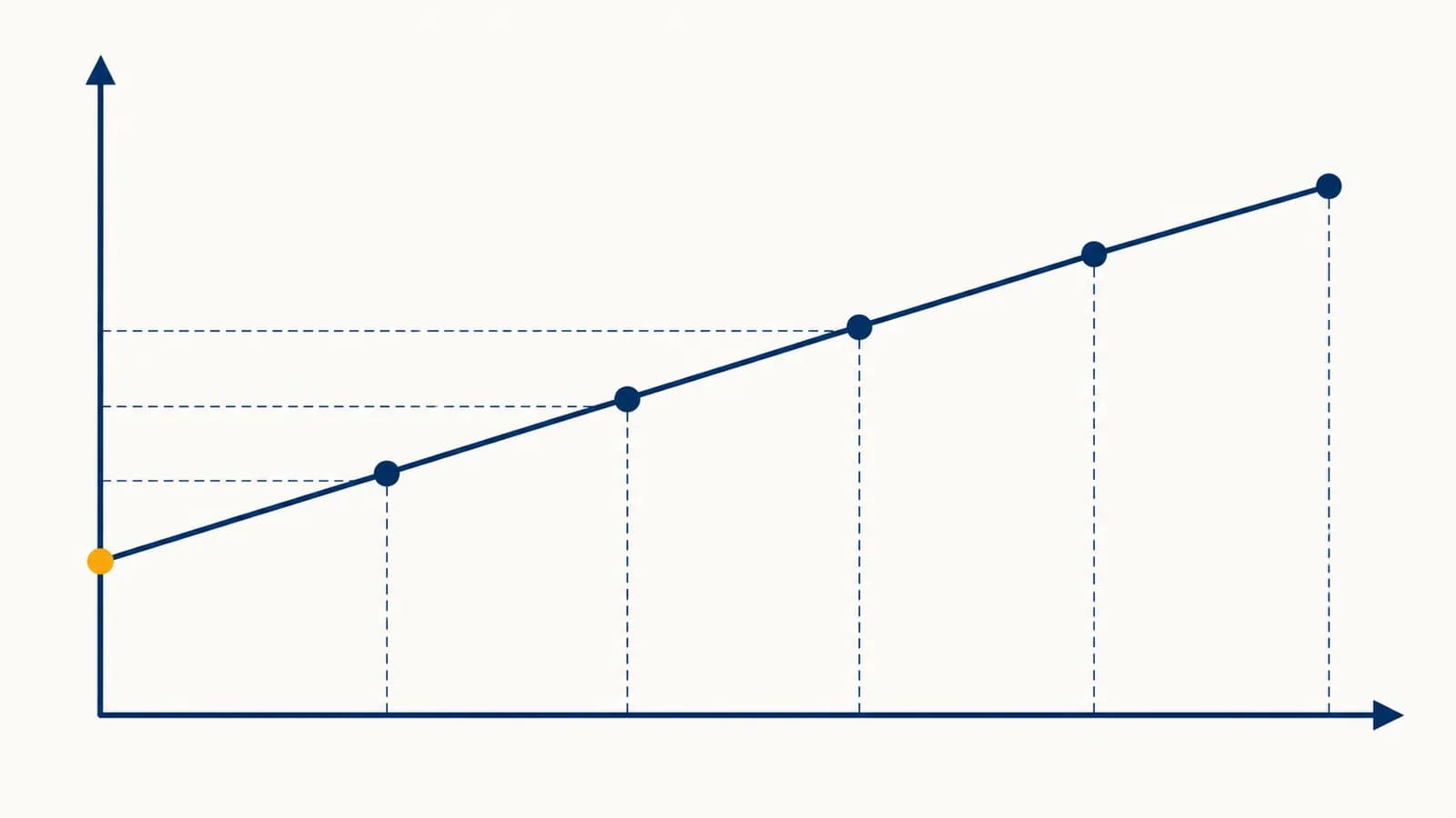
A linear function is a mathematical rule that produces a constant rate of change between two quantities, in the context of algebra and coordinate geometry. Its equation is usually written , where the slope gives the rate of change and the -intercept gives the starting value. The graph of a linear function is a straight line. Linear functions exist because many useful relationships can be described, or closely estimated, by adding the same amount whenever an input increases by one unit.
What a linear function actually is
A linear function assigns exactly one output to each allowed input and changes its output by a constant amount over equal input intervals. In the coordinate plane, that constant change makes all of its points lie on one straight, nonvertical line.
A function is a rule connecting an input, usually called , to one output, usually called . If produces , the ordered pair records that input and output together. A collection of such pairs is linear when the output differences stay proportional to the input differences.
Consider . Starting with an input of zero gives an output of five. Increasing the input by one always adds two to the output:
| Input | Calculation | Output | Change in output |
|---|---|---|---|
| 0 | 5 | ||
| 1 | 7 | ||
| 2 | 9 | ||
| 3 | 11 |
The same pattern works between any two inputs, not only consecutive whole numbers. If the input rises by , the output rises by . If the input falls by four, the output falls by eight. This fixed ratio is what makes the relation linear.
Constant rate test: a function is linear if has the same value for every pair of distinct inputs in its domain.
The word linear sometimes gets used more narrowly in advanced mathematics, where a truly linear map must send zero to zero. School algebra usually includes equations such as under the name linear functions, even though mathematicians may call them affine functions. On this page, the standard school meaning applies.
How slope and intercept work together
Slope controls how much the output changes per unit of input, while the intercept sets the output when the input is zero. Together they fix one and only one nonvertical line, expressed by the slope intercept form .
For , the slope is and the vertical intercept is .
The coefficient is a rate with units. In a taxi model where is distance in kilometres and is total price in dollars, a slope of means 2.50 dollars per kilometre. The intercept has the output's units, dollars in this case, and represents the fare before any distance is travelled.
The size of the slope measures steepness only after the axis scales and units are known. A slope of is not automatically steep on a graph whose vertical tick marks count by thousands. Changing kilometres to metres also multiplies a numerical rate by a conversion factor without changing the physical relationship.
The intercept is a starting value only when zero is a meaningful input. In a model of adult height against age, the fitted vertical intercept might be the height predicted at age zero, far outside the ages used to build the model. It still positions the line algebraically, but it should not be treated as a sensible measurement.
How to build a linear equation from information
A linear equation can be built by identifying a constant rate and one known input output pair. Calculate the slope first, substitute the known point into to find the intercept, then check the finished rule against the original information.
Decide what the input and output measure. This prevents a rate such as dollars per hour from being reversed into hours per dollar.
For two points, divide the change in output by the change in input: .
Put one point and the slope into , then solve for .
Substitute the other known pair. Matching it catches sign errors and reversed subtraction.
Suppose a water tank contains 620 litres at 9:00 and 500 litres at 11:00 while a pump drains it steadily. Let be hours after 9:00 and be litres. The two points are and .
Since when , the equation is .
The negative slope matches the physical action: the tank is losing water. At 11:00, , so the equation gives . It passes the check. Setting also predicts when the tank empties: , so hours after 9:00, provided the steady rate continues.
If the wording gives a starting amount and a per unit change directly, less work is needed. A 40 dollar service fee plus 18 dollars per hour translates to . This is closely related to the constant multiplier reasoning developed in how ratios and proportions connect quantities, with an added starting value.
How a graph, table, equation, and description represent the same rule
A graph, a table, an equation, and a verbal description can encode the same linear function. Each form emphasizes different information: graphs show overall direction, tables show selected pairs, equations allow calculation, and descriptions supply meaning and units.
Take a candle that begins 24 centimetres tall and burns down by 1.5 centimetres each hour. The description gives an initial height of 24 centimetres and a rate of centimetres per hour. With time and height , the equation is .
A table might list , , , and . Plotting those points gives a descending straight line. The plotted segment should stop at the point where the candle reaches zero, because negative candle height has no meaning here. The algebraic rule accepts more inputs, but the physical model does not.
Moving between representations is more than a classroom conversion exercise. A manager may receive costs in a table, see a trend on a chart, and need an equation for a budget. A scientist may begin with a proposed equation and graph residuals to test whether it describes measurements adequately. The form changes, while the relation between the quantities stays the same.
Graphing also exposes impossible interpretations. If a quantity cannot be negative, the meaningful part of the graph must remain on or above the horizontal axis. If time is recorded only after an event begins, negative inputs are excluded. A correct equation can still be used incorrectly when its domain is ignored.
Linear functions versus proportional relationships
A proportional relationship is a special linear function with a zero intercept, so its equation has the form and its graph passes through the origin. A general linear function may include a nonzero fixed starting amount .
. Zero items cost zero dollars, and doubling the number of items doubles the total cost. The graph passes through .
. A fixed 7 dollar charge remains when the item count is zero. Doubling the item count does not double the whole total.
The distinction matters whenever a fixed fee, baseline measurement, or initial stock is present. A gym bill with a joining fee and a monthly charge is linear over a suitable period, but it is not proportional. A car travelling at constant speed from a location 20 kilometres east of a marker has position ; its position is linear in time but not proportional to time.
One quick test is to evaluate the rule at zero. If , a linear function is proportional. If , it is not. Another test is to compare for nonzero inputs. That quotient stays constant for proportional relationships, but not for lines with nonzero intercepts.
Linear functions versus nonlinear functions
A linear function has one constant slope, while a nonlinear function changes rate or direction. Equal steps in input produce equal output changes only in the linear case; curved graphs, variable first differences, products of variables, and powers such as signal nonlinearity.
Compare with . For inputs 0, 1, 2, and 3, the outputs of are 1, 4, 7, and 10. Their first differences are always 3. The outputs of are 1, 2, 5, and 10. Their first differences are 1, 3, and 5, so the rate is changing.
The graph of bends because its slope is not fixed. This is the kind of changing rate studied through equations whose graphs form parabolas. Exponential functions change by equal factors over equal input steps, while linear functions change by equal amounts. That difference separates steady addition from repeated multiplication.
A line of best fit is still a model. Real data points do not need to sit exactly on one line for a linear approximation to be useful, but the departures from the line must be examined before trusting predictions.
A curved process can look almost linear across a short interval. The surface of Earth, for example, looks flat over a small patch even though Earth is not flat. In the same way, a changing relationship may be approximated with a tangent line or a fitted line over a restricted range. The approximation is useful only while its error remains acceptable for the decision being made.
How linear functions show up in money, work, and measurement
Linear functions appear when a total combines a fixed amount with a constant charge, earning rate, conversion factor, or steady change. They model wages, simple pricing plans, unit conversions, depreciation estimates, inventory movement, and many short range physical processes.
A freelance repair technician charges a 55 dollar visit fee and 32 dollars for each half hour of labour. If counts half hour blocks, the labour bill is . Three blocks cost dollars.
The equation separates two business facts. The slope is the charge for each additional block. The intercept is the charge that does not depend on the number of blocks. A competing technician with equation starts cheaper but rises faster. Set the bills equal to find the break even job length:
At five half hour blocks, both bills are dollars.
Before that point, the second technician costs less; after it, the first does. This is how an intersection of two lines becomes a decision threshold. The same method compares mobile plans, rental offers, manufacturing methods, and any pair of options with fixed and variable costs.
Unit conversion supplies exact linear functions. Celsius temperature converts to Fahrenheit temperature through . The multiplication changes the size of each degree, and the added 32 aligns the two scales' zero points. Because of the offset, temperature conversion between these scales is linear but not proportional.
Some money calculations are only linear under stated assumptions. Straight line depreciation assigns an asset the same loss of book value each year, but market value rarely falls so neatly. Simple interest grows linearly when interest is calculated only on the original principal. Compound interest is nonlinear because each period's interest changes the base used for the next period.
Measurement devices often use a linear calibration over an operating range. A sensor may turn voltage into temperature using a fitted slope and intercept. The technician must check units, calibration limits, and residual error. A line that matches readings between two tested temperatures does not automatically describe behavior outside those temperatures.
4 mistakes people make with linear functions
Most errors with linear functions come from confusing a rate with a starting value, reversing the slope calculation, ignoring units or domain, or assuming any visible trend must continue. Each mistake changes the meaning of the equation, not only its arithmetic.
1. Reversing rise and run
Slope is output change divided by input change. If is time in hours and is distance in kilometres, has units of kilometres per hour. Reversing it gives hours per kilometre, which is a different rate.
Subtraction order may be chosen either way, but it must stay consistent. For points and , . Reversing both differences gives as well. Reversing only one produces the wrong sign.
2. Treating the intercept as the slope
In , 6 is the per unit change and 40 is the output at zero. The intercept does not tell how fast the output changes. Labeling units makes the roles visible: 6 might be dollars per ticket, while 40 is dollars.
3. Ignoring the meaningful domain
A formula may accept inputs that the situation forbids. If models a delivery containing boxes, negative values and fractional boxes may be invalid. The practical domain could be whole numbers beginning at zero, even though the drawn line contains every real input.
4. Extending the line without evidence
A steady pattern inside observed data does not guarantee the same pattern forever. A worker paid hourly may reach an overtime threshold. A tank stops draining once empty. A subscription may change price. Extrapolation assumes that the mechanism stays constant, so the assumption must be defended.
This sentence is a useful check before writing an equation. Ask what physical, financial, or procedural mechanism keeps the rate fixed. If there is no such mechanism, the line may still summarize a narrow range, but it should not be mistaken for a permanent law.
How vertical and horizontal lines fit the picture
A horizontal line is a linear function with slope zero, while a vertical line is not a function of . The difference comes from output assignment: a vertical line gives one input many outputs, violating the definition of a function.
The equation assigns the output 5 to every input. Its graph is horizontal, its slope is zero, and it fits with and . A constant function is therefore linear in the school algebra sense.
The equation includes every point whose horizontal coordinate is 5. One input is paired with many possible values, so it fails the vertical line test. Its slope would require division by zero, which is undefined. The line is straight, but it is not a function of .
What domain, range, zeros, and intersections tell you
Domain lists allowed inputs, range lists possible outputs, a zero marks where the output is zero, and an intersection marks where two relations have the same input and output. These features translate algebraic points into limits, thresholds, and comparisons.
For , solve to get the zero . The graph crosses the horizontal axis at . Depending on context, that point might mean a debt is repaid, a reservoir is empty, or profit moves from negative to positive.
A nonconstant linear function with all real inputs also has all real outputs. A real situation usually narrows both sets. If a machine fills containers for no more than eight hours, the domain might be . The range then comes from evaluating the line at those boundary inputs, with direction determined by the sign of the slope.
Intersections solve systems. If income is and cost is , equality gives , so . At 20 units, both totals are 300 dollars. Below that quantity cost exceeds income; above it income exceeds cost.
How interpolation and extrapolation use a line
Interpolation estimates between known inputs, while extrapolation predicts beyond them. A linear model can do both by substituting a new input, but interpolation is usually safer because extrapolation assumes the same rate continues into an unobserved region.
Suppose a container holds 18 litres at two minutes and 42 litres at six minutes while filling steadily. The slope is litres per minute. Substituting gives . Estimating the volume at four minutes is interpolation: litres.
Predicting the volume at twenty minutes is extrapolation. The equation gives 126 litres, but that answer is useful only if the container has enough capacity and the filling rate remains fixed. The arithmetic is correct under the model. The prediction may still be physically false.
Interpolation uses nearby evidence on both sides of the estimate. A straight line may still be imperfect, but the estimate stays within tested conditions.
Extrapolation has evidence on only one side. Capacity limits, changing rates, and new rules can make the continued line fail.
Data may also contain decimals that need careful interpretation before fitting or reading a line. The techniques in working accurately with fractional and decimal values help preserve units and avoid rounding too early. Keep extra precision during the calculation, then round the final result to a level supported by the measurements.
A linear model turns constant change into a usable prediction
Linear functions connect algebra to observable change by pairing a starting value with a constant rate. They let you calculate missing values, compare options, locate thresholds, and test whether a straight line is a defensible model for a real process.
The habit to keep is simple: name the quantities, attach units, locate the starting value, and ask what makes the rate constant. Then test the equation against known points and restrict it to inputs the situation permits. These checks turn symbols into an accountable description of what is happening.
The takeaway: read as a mechanism. Begin at , add for each one unit increase in , and stop trusting the rule when the constant rate assumption stops matching reality.
Linear functions sit near the entrance to algebra because the same ideas lead onward to systems, inequalities, data models, and calculus. To place this topic beside those connections, see how the mathematics guides fit together. Then notice one changing quantity today and ask whether equal input steps really produce equal output changes.