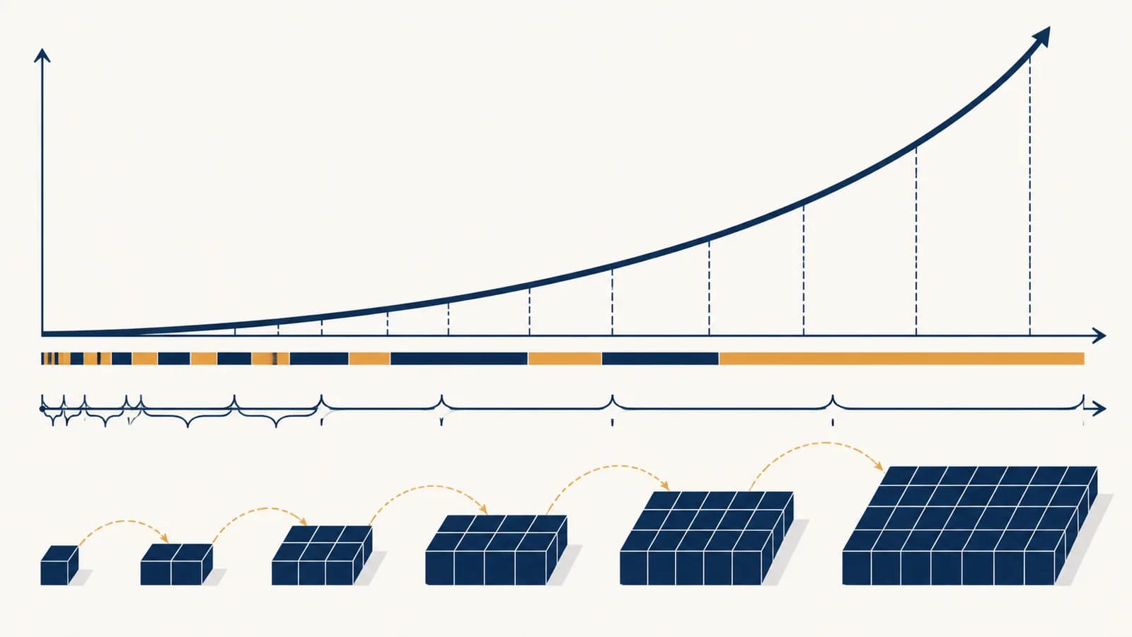
Exponents describe repeated multiplication
Exponential growth happens when a quantity changes by the same factor over equal intervals, and logarithms tell you how many intervals that change takes. By the end, you can model growth, compare rates, estimate doubling time, and read logarithmic scales without treating either idea as a mysterious calculator button.
An exponent is shorthand for repeated multiplication. In , the base is 2 and the exponent is 5, so the expression means . The exponent counts how many copies of the base are multiplied together. This is different from , which means repeated addition and equals 10.
A plant grows by 3 centimetres each week. Its height follows a straight line because every week contributes the same difference.
A culture grows by 3 percent each hour. Each increase is based on the new total, so the amount added changes over time.
The distinction between a constant difference and a constant factor controls the model. Linear change has the form , where is added each interval. Exponential change has the form , where multiplies the quantity each interval. If is greater than 1, the quantity grows. If lies between 0 and 1, the quantity decays.
A starting amount of 500 growing by 4 percent per period becomes after three periods.
Here is the starting amount, is the rate written as a decimal, and is the number of equal periods. A 4 percent increase gives a growth factor of . A 4 percent decrease gives a decay factor of . The sign of the rate matters, but the multiplication factor does the actual work.
Why does percentage growth speed up?
Percentage growth speeds up because each new percentage is calculated from a larger total. The rate can stay fixed while the absolute increase rises. This feedback is compounding: growth from earlier periods becomes part of the base used to calculate later growth.
Suppose a savings balance starts at 1,000 units and earns 10 percent per year, with the return added once each year. The first increase is 100, producing 1,100. The next increase is 10 percent of 1,100, so it is 110. The third is 121. The percentage never changes, but the amount added does.
For the first year, the current balance is 1,000.
Ten percent of 1,000 is 100, so the new balance is 1,100.
Ten percent of 1,100 is 110. Compounding means the base is updated after each interval.
This mechanism appears in savings, debt, populations, radioactive decay, cooling models, and the spread of information. The surrounding science or economics determines whether the rate can remain stable. The mathematics only states what follows if the factor stays fixed for the intervals being studied.
The totals come directly from . They also show why adding 10 percent three times is not the same as adding 30 percent once. A single 30 percent increase produces 1,300, while three compounded increases produce 1,331. The extra 31 is growth earned on earlier growth.
Real populations rarely follow one exponential curve forever. Food, space, disease, migration, and policy all affect the rate. Maps of how population density varies across places add information that a single growth percentage cannot show. A model becomes useful when its assumptions match the question, not when its curve looks impressive.
How can you tell linear and exponential change apart?
Equal differences signal linear change, while equal ratios signal exponential change. Subtract consecutive values first. If those differences are constant, try a linear model. If they are not, divide consecutive values. A constant ratio supports an exponential model over those observations.
| Time | Sequence A | Change in A | Sequence B | Ratio in B |
|---|---|---|---|---|
| 0 | 5 | 5 | ||
| 1 | 8 | +3 | 10 | 2 |
| 2 | 11 | +3 | 20 | 2 |
| 3 | 14 | +3 | 40 | 2 |
Sequence A is . Sequence B is . At first, both may look modest. Later, repeated doubling outruns repeated addition because every existing unit contributes to the next increase.
A rising curve is not automatically exponential. A quadratic curve, a changing seasonal pattern, or several joined linear trends can also bend upward. Test differences, ratios, and the mechanism behind the data.
Noisy measurements make the test less tidy. Ratios may hover around a value instead of matching it exactly. In that case, a fitted model can describe an approximate trend, but residuals must be checked. A residual is the observed value minus the model's predicted value. A visible pattern in the residuals is evidence that the model is missing structure.
Units also expose mistakes. A rate of 5 percent per month cannot be inserted as 5 percent per year without conversion. The exponent counts intervals, so the time unit in must match the time unit attached to the rate. Twelve monthly increases give , not .
Logarithms answer the missing exponent question
A logarithm gives the exponent needed to produce a number from a chosen base. The statement means exactly the same thing as . Exponents build a result; logarithms work backward from the result to the exponent.
For example, , so . Likewise, , so . The base matters. , while , because 2 must be multiplied by itself six times to make 64, but 8 needs only two copies.
Two bases appear often. The common logarithm uses base 10 and is written on many calculators. The natural logarithm uses the constant , approximately 2.718, and is written . Natural logarithms fit processes modelled with continuous change, but any logarithm base can solve an exponential equation if used consistently.
To find when 500 growing at 4 percent reaches 800, calculate periods.
The algebra explains the formula. Divide both sides by to isolate the power. Take a logarithm of both sides. Then use the rule , which brings the exponent down as a multiplier. Division finally isolates .
A logarithm therefore measures multiplicative distance. Ordinary subtraction asks how much must be added to move from one value to another. A logarithm asks how many equal multiplication steps separate them. That is exactly the missing information in doubling time, decay time, and threshold problems.
What does doubling time reveal?
Doubling time is the number of equal intervals required for an exponentially growing quantity to become twice its starting size. It depends on the growth factor, not on the initial amount. Logs calculate it exactly by solving .
The formula is . At 5 percent growth per interval, intervals. Starting with 20 or 20,000 changes the doubled amount, but it does not change the time required under the same fixed rate.
A laboratory culture begins with 600 cells and grows by 5 percent per hour under stable conditions. Its doubling time is about 14.21 hours, so the model predicts about 1,200 cells then. The calculation is a conditional prediction, because nutrients and space may later alter the rate.
For modest percentage rates, the Rule of 70 gives a useful mental estimate: divide 70 by the percentage growth rate. At 5 percent, it predicts about 14 intervals, close to the logarithmic result. It is an approximation, not an identity. The exact formula should be used when precision affects a decision.
Half-life is the decay version of the same idea. If a quantity keeps a fraction each interval, with , its half-life solves . Thus . Both logarithms are negative, so their ratio is positive.
This perspective helps in environmental planning. A resource that grows slowly can be overtaken by demand that doubles faster. The physical difference between stocks that replenish and stocks that do not is developed in the geography of renewable and non-renewable resources. The equation can compare rates, but evidence about the actual resource determines which rate belongs in it.
Why do logarithmic scales compress large ranges?
A logarithmic scale places equal ratios at equal distances, so multiplication replaces addition as the visual step. Values such as 1, 10, 100, and 1,000 are evenly spaced on a base 10 log scale because each is ten times the previous value.
On an ordinary linear axis, the distance from 1 to 10 is 9 units, while the distance from 100 to 1,000 is 900 units. The larger values dominate the plot. On a base 10 logarithmic axis, their positions are 0, 1, 2, and 3 because those are their logarithms. Each tenfold change occupies the same width.
Equal distances represent equal differences. Moving one grid step might add 10 every time.
Equal distances represent equal ratios. Moving one grid step might multiply by 10 every time.
This compression makes it possible to display quantities that span many orders of magnitude. An order of magnitude is a factor of ten. A change from 100 to 1,000 is one order of magnitude; a change from 100 to 10,000 is two.
Logarithmic scales also change the shape of exponential data. Taking logs of gives . This is a straight-line equation in . A straight pattern on a graph with a logarithmic vertical axis can therefore support an exponential model.
Read the tick labels before reading the slope. On a logarithmic axis, equal vertical gaps do not mean equal numerical increases. They mean equal multiplication factors.
Some familiar scientific scales use logarithmic ideas, but their definitions are not interchangeable. Acidity measured by pH relates to hydrogen ion activity through a negative base 10 logarithm. Sound level in decibels uses a logarithmic ratio with a defined reference. The mathematics compresses ratios in both cases, while the scientific definition supplies the quantity and convention.
Where do exponential models break?
An exponential model breaks when its multiplication factor does not remain reasonably stable. Finite food, limited space, changing interest rates, medical treatment, regulation, and human behaviour can all alter the process. Extrapolating beyond observed conditions can then produce confident but unsupported numbers.
A population with abundant resources may grow close to exponentially for a time. As crowding increases, births, deaths, and movement can change. A logistic model represents one possible slowdown by including a carrying capacity, but even that capacity can shift with climate, technology, or habitat damage.
Here is the modelled carrying capacity, controls growth, and reflects the starting condition.
The curve initially may resemble exponential growth, then bends as it approaches . This does not mean every real population settles neatly at one ceiling. It means the model encodes a slowing mechanism that a pure exponential equation lacks.
Environmental systems give especially clear warnings about fixed-rate assumptions. Loss of vegetation can expose soil, which reduces water retention and makes plant recovery harder. The feedbacks described in the causes and effects of desertification can change direction and strength over time. One constant exponent cannot represent every stage.
Ask what is being multiplied and why the factor might stay similar from one interval to the next.
Confirm that the rate and the time variable use the same interval.
Compare predictions with observations and inspect residuals for a pattern.
State the conditions under which the rate was observed and avoid extending it past known changes without evidence.
Graphs can mislead before any calculation begins. A truncated time window can hide a slowdown. A logarithmic axis can make a steep rise look gentle. A fitted curve can pass close to old data and still fail on new data. Labels, units, time range, and assumptions are part of the argument.
This habit of checking place, resources, and scale belongs naturally within geographical study of connected human and physical systems. Mathematics supplies a structure for the pattern. Subject knowledge tells you what the variables mean and what forces can change them.
Exponents build growth, and logarithms make it readable
Exponents express repeated multiplication, while logarithms recover the exponent hidden inside a result. Together they convert changing quantities into questions you can answer: what factor acts each interval, how long a threshold takes, and whether a graph supports the proposed mechanism.
When a quantity changes, begin by checking differences and ratios. Constant differences suggest a linear model. Roughly constant ratios suggest an exponential one. Write the rate as a factor, keep the time units consistent, and use a logarithm when time appears in the exponent.
The takeaway: Exponential growth is repeated multiplication, not a synonym for “very fast.” A logarithm measures how many multiplication steps produced a result. Both ideas are powerful only when the rate, units, and real-world limits are stated clearly.
A good model does more than produce a number. It makes its assumptions visible enough to test. Once you can move between and , large changes stop looking like walls of zeros. They become factors, intervals, and conditions that can be checked.