What makes a quantum computer different?
Quantum computing represents and transforms information using quantum states, then extracts a classical answer by measurement. Its advantage is not that it tries every answer at once. It comes from shaping probability amplitudes so useful answers become more likely.
Ordinary computers store bits. Each bit is recorded as one of two values, 0 or 1. Quantum computers use quantum bits, called qubits. A qubit can be prepared in a state described by two amplitudes, one attached to 0 and one attached to 1. Those amplitudes can combine, cancel, and become correlated with the amplitudes of other qubits.
This gives quantum programs a different set of moves. A classical program changes definite bit values through logic gates. A quantum program applies carefully chosen operations to amplitudes. Measurement then produces ordinary bits, which are the only results a person or classical computer can read directly.
Knowing that mechanism makes it possible to explain qubits, interference, entanglement, algorithms, and error correction in concrete terms. It also gives you a practical test for judging claims about quantum speed: identify the pattern being used and how measurement reveals it.
A quantum computer checks every possible answer in parallel and reveals the best one.
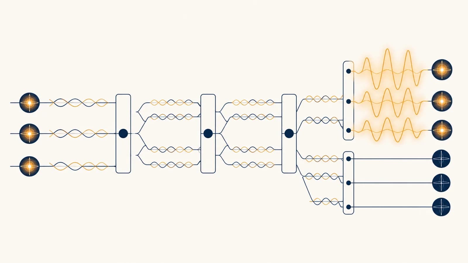
A quantum circuit changes amplitudes so that measurement is more likely to return a useful result. Most of the state remains hidden.
That distinction explains both the promise and the limits. A collection of qubits can be described using many amplitudes, but measurement does not print the whole description. A useful quantum algorithm must arrange interference before measurement. Otherwise, the final bits look like an unhelpful random sample.
How can a qubit be both 0 and 1?
A qubit is not literally two classical values at once. Before measurement, its state is a weighted combination of the basis states 0 and 1. The weights are amplitudes, and their squared magnitudes determine the probabilities of measured outcomes.
A common notation writes a single qubit as follows. The symbols and name the two basis states. The coefficients and may be complex numbers, which means they carry both magnitude and phase.
If and , measurement returns 0 with probability and 1 with probability .
The requirement that the probabilities add to 1 is familiar mathematics. The strange part is that amplitudes, rather than probabilities, are transformed during a computation. Two paths with opposite phases can cancel even when each path alone would have produced a possible outcome.
Superposition is best understood as a rule for predicting measurement results, not as a tiny switch with a secret classical setting. Repeating the same preparation and measurement many times reveals its probability pattern. The connection to probability and counting methods is direct, but quantum amplitudes add an extra layer because phase controls interference.
Measurement changes the situation. Measuring a qubit in the 0 and 1 basis returns one value and leaves the qubit in the corresponding basis state. The original amplitudes cannot be recovered from that single result.
Other measurement bases are possible. A qubit that is perfectly predictable in one basis can be evenly split in another. This is why phrases such as “the qubit is 0” are incomplete unless the preparation and measurement basis are specified.
Why does interference do the real computational work?
Interference lets a quantum circuit increase some outcome amplitudes and reduce others. The circuit creates several computational paths, changes their phases, and recombines them. A successful algorithm makes paths leading toward useful evidence reinforce while unwanted paths tend to cancel.
Picture waves meeting on water. Two crests reinforce; a crest and a trough cancel. Quantum amplitudes follow related addition rules, although they are mathematical quantities rather than water waves. If an algorithm creates many branches but never recombines them intelligently, superposition alone provides no useful speed.
The Hadamard gate gives a compact example. Applied to , it produces equal amplitudes for 0 and 1. Applied again immediately, it returns the qubit to . The two applications do not create more randomness. Their paths recombine, and the amplitude for 1 cancels.
Real algorithms use longer versions of this pattern. They encode a property of a candidate answer into phase, then use more gates to turn phase differences into measurable probability differences. Pattern recognition matters here: the programmer looks for symmetry, repetition, periodicity, or another structure that interference can expose.
What changes when qubits become entangled?
Entangled qubits have a joint state that cannot be split into independent states for each qubit. Their measurement results can show correlations that no assignment of separate local quantum states reproduces, yet those correlations cannot send a controllable message faster than light.
Two qubits have four basis outcomes: 00, 01, 10, and 11. A particular entangled state can assign equal amplitudes to 00 and 11 while assigning zero amplitude to the other two. Each qubit alone looks random, but measuring both in the same specified basis produces matching results.
Measurement in the computational basis returns 00 or 11, each with probability . It never returns 01 or 10.
Entanglement makes the whole register the natural unit of description. For qubits, there are basis strings. That exponential state description is powerful, but it is not an exponential readout channel. Measurement still returns one bit string per run.
The sequence follows the same doubling pattern taught in exponents and powers. Each additional qubit adds a binary choice to every existing basis string. Quantum gates can act on this joint structure without listing every amplitude in ordinary memory, but only specially designed algorithms turn that fact into fewer computational steps.
How does a quantum program produce a trustworthy answer?
A quantum program prepares qubits, applies gates in a fixed circuit, measures them, and repeats the circuit to estimate an outcome distribution. Classical software chooses parameters and checks results. Trust comes from repeated trials, calibration, mathematical guarantees, and comparison with known cases.
A circuit is closer to a controlled experiment than to a conventional script. It does not usually print a stable answer after one run. A single measurement is a sample. Repeated runs, often called shots, estimate how frequently each output appears.
Reset qubits to a known starting state so repeated trials have the same conditions.
Apply gates that encode the input and arrange interference around the property being tested.
Convert selected qubits into classical bits. This gives one sample from the circuit's output distribution.
Collect enough samples to estimate the pattern, then test the candidate result with classical computation when possible.
Suppose an ideal circuit should return 1 with probability . In 100 runs, exactly 75 ones are not guaranteed. Sampling fluctuates. More runs usually narrow the uncertainty in the estimated proportion, while hardware errors can introduce a separate bias that repetition alone does not remove.
Building the surrounding system therefore requires ordinary testing, compilers, device control, data analysis, and monitoring. The principles of turning software prototypes into production systems still apply. A quantum processor is one specialized component inside a larger classical machine.
A research team tests a small chemistry circuit. They first run circuits with known answers, compare results across qubit layouts, record calibration data, and simulate a reduced version classically. Only then do they treat an unfamiliar output as evidence rather than as a mysterious number produced by the device.
This hybrid structure is common because classical machines are excellent at bookkeeping, optimization, and verification. Quantum hardware is reserved for the part of a method that can use interference or entanglement. The split may change as devices improve, but checking the output remains part of sound computation.
Which problems can quantum algorithms actually change?
Quantum algorithms can reduce the number of steps for certain structured problems, including integer factoring, unstructured search, and simulation of quantum systems. They do not accelerate every program, and a formal speed advantage may still be impractical once input, error correction, and verification are counted.
Shor's algorithm uses period finding to factor integers in polynomial time on an ideal fault-tolerant quantum computer. This matters because widely used public key systems such as RSA rely on the practical difficulty of factoring large integers with known classical methods. The algorithm is mathematically established; running it against cryptographic key sizes requires machines far beyond small demonstrations.
Grover's search algorithm offers a different kind of improvement. Searching an unstructured set of possibilities takes on the order of quantum queries, compared with classical checks in the basic black box model. That is a quadratic improvement, not an instant answer.
A visible search comparison: if a black box hides one marked item among 1,000,000 possibilities, the basic counts scale like 1,000,000 classical checks versus about quantum queries. Real running time also includes circuit costs and error handling.
Quantum simulation is a more natural match. Molecules and materials already obey quantum rules, so representing their states on classical machines can become expensive as the modeled system grows. A quantum processor may represent selected quantum interactions more directly. Useful results still depend on accurate models, suitable algorithms, and controlled errors.
Optimization and machine learning attract attention, but broad claims need care. A quantum method may be faster under a particular input model or mathematical promise without beating the best classical system on useful data. Input loading can consume the expected gain. A fair comparison specifies the task, error tolerance, hardware assumptions, and total cost.
The safest question is not “Can quantum computing solve this?” It is “What repeated structure does the algorithm exploit, how does interference reveal it, and what must be paid to prepare and verify the result?” Those questions separate a computational mechanism from a marketing claim.
Why are useful qubits so difficult to build?
Useful qubits must be initialized, controlled, connected, and measured while remaining isolated from unwanted interactions. Heat, stray fields, imperfect pulses, and material defects disturb amplitudes and phases. Quantum error correction can suppress these faults, but it requires many coordinated physical operations.
Classical error correction can copy bits and compare copies. An unknown quantum state cannot be copied perfectly, a restriction called the no cloning theorem. Quantum error correction works around this by spreading information across entangled physical qubits and measuring carefully chosen error indicators called syndromes. These checks reveal the type of error without directly reading the protected logical state.
A controllable quantum device, such as a superconducting circuit or trapped ion. Its state is exposed to imperfect operations and environmental noise.
Quantum information encoded across several physical qubits so errors can be detected and corrected while the computation continues.
Error correction does not require flawless components. It requires physical error rates below the threshold of a chosen code and enough extra hardware to repeat syndrome checks. The exact overhead depends on the code, device, circuit, and target reliability, so one universal conversion between physical and logical qubits would be misleading.
Different hardware platforms make different trades. Superconducting circuits can use fast electrical control but require very low temperatures. Trapped ions can offer long lived states and precise control, while gate speed and connectivity present engineering constraints. Photonic approaches use particles of light and face their own demands for sources, routing, loss control, and detection.
This is why qubit count alone says little about capability. Connectivity affects how many extra gates are needed. Gate fidelity affects how long a circuit can run. Measurement quality, reset speed, compiler choices, and logical error rates all affect the useful work a machine can complete.
Quantum literacy is practical pattern recognition
Quantum literacy means tracing a claim through four questions: what state is prepared, what pattern the gates encode, how interference changes the output distribution, and how measurement supports the conclusion. Those questions let a curious reader evaluate real uses without pretending the engineering is simple.
They also expose common category mistakes. A quantum computer is not a faster replacement for every laptop. Entanglement is not a communication channel. Superposition is not a readable list of every answer. An algorithmic speedup on an ideal machine is not the same as a lower bill on existing hardware.
The best foundation is mathematical rather than mystical. Vectors describe states, matrices describe gates, complex numbers track phase, and probability connects amplitudes to observations. The broader mathematics foundations behind computation make each mechanism more concrete and easier to check.
The takeaway: Look for the pattern a quantum algorithm uses, the interference that makes the pattern visible, and the measurement process that turns it into evidence. If any link is missing, the claim is incomplete.
Curiosity is enough to begin because the central habit is already familiar: follow the information. Identify what is represented, what operation changes it, and what observation can confirm the change. Quantum computing uses unfamiliar rules, but it still rewards precise definitions, visible arithmetic, and careful tests.