The Algebra Behind Every Pricing Decision

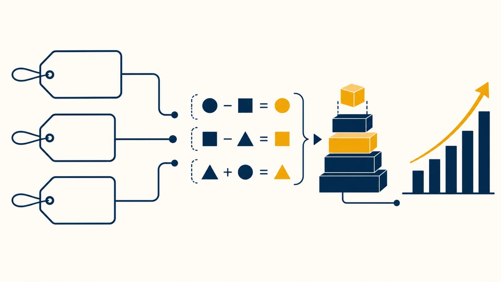
How does algebra turn a cost into a price?

Every pricing decision is an algebra problem: a seller chooses a price, subtracts the costs attached to the sale, and tests how customer demand changes the result. Once the variables are visible, pricing formulas for markup, margin, discounts, and break-even sales become understandable and checkable.

The simplest model has three quantities. Let $C$ be the cost of supplying one unit, $M$ be the money added above that cost, and $P$ be the selling price. The relation is addition, but writing it symbolically makes it reusable for a sandwich, a haircut, a concert ticket, or a software subscription.

Letters do more than shorten the arithmetic. They let a seller rearrange the same relationship. If the market will accept a price of $60 and the desired addition is $20, the maximum unit cost is found with $C = P - M$. This is the same habit taught in mathematical reasoning across the school curriculum: name unknown quantities, state their relationship, then solve for the quantity that matters.

A real pricing model repeats this process rather than stopping after the first addition. The price affects how many units people buy. The sales quantity determines how widely fixed costs are spread. Fees, returns, and discounts change the money kept from each order. Algebra connects those moving parts without pretending that any one of them is fixed forever.

Why are markup and margin not the same?

Markup measures profit relative to cost, while gross margin measures gross profit relative to selling price. They use the same money difference but divide by different bases, so a 50% markup does not mean a 50% margin.

Use the $40 cost and $60 price. Gross profit per unit is $20. Dividing $20 by the $40 cost gives a 50% markup. Dividing the same $20 by the $60 price gives a gross margin of one third, or about 33.3%. Nothing about the transaction changed. Only the comparison base changed.

The distinction matters when the target is stated as a percentage. Suppose a seller wants a 40% gross margin and unit cost is $30. Adding 40% of cost would give $42, but that price produces only about a 28.6% margin. The correct equation makes cost equal to the part of price that is not margin: $C = P(1-g)$, where $g$ is the target margin rate. Solving gives $P = \frac{C}{1-g}$. With these values, $P = \frac{\$30}{1-0.40} = \$50$.

Businesses may define cost differently. One calculation may include only the item bought from a supplier. Another may also include packaging, payment fees, and shipping paid by the seller. The algebra can be correct while the answer is misleading because a cost was omitted. Good variable definitions are part of the calculation, not paperwork added afterward.

What price covers all costs?

A price covers all costs only when total revenue equals or exceeds fixed costs plus variable costs. Break-even analysis finds the sales quantity where profit is zero, using the contribution from each sale to pay down fixed costs.

Fixed costs do not change directly with the next unit sold within the modelled range. A monthly equipment rental is one example. Variable costs rise with sales volume, such as ingredients used in each meal. If $F$ is fixed cost, $v$ is variable cost per unit, $p$ is price per unit, and $q$ is quantity sold, profit can be written as follows.

The difference $p-v$ is the contribution per unit. It is not the final profit on that unit, because fixed costs still need to be paid. Once total contribution equals fixed cost, the model reaches break-even. After that quantity, each additional unit adds its contribution to profit, provided the assumptions still hold.

This model also works backward. If the stall expects to sell only 80 meals, it can solve for the price needed to break even: $p = v + \frac{F}{q}$. The answer is $\$8 + \frac{\$1{,}200}{80} = \$23$. That does not prove customers will pay $23. It identifies the price required under the stated volume and cost assumptions.

Software performs these calculations at scale, but the structure still begins with variables and expressions. The ideas behind variables and step-by-step program logic explain how a pricing rule becomes code: store the inputs, apply the equation, test the output, and repeat when an input changes.

How do discounts and taxes combine?

Successive percentage changes multiply rather than add because each percentage acts on a new base. A 20% discount followed by a 10% discount leaves 72% of the original price, so the combined discount is 28%, not 30%.

A discount rate $d$ leaves the fraction $1-d$ of a price. Starting with list price $L$, two discount rates $d_1$ and $d_2$ produce a final price found by multiplying both remaining fractions.

The second discount is only $8 because it applies to the reduced $80 price. This is a general rule of percentage change. A rise of 20% followed by a fall of 20% also fails to return to the starting value: $1.20 \times 0.80 = 0.96$, leaving 96% of the original amount.

Taxes use the same multiplier idea. If a tax rate $t$ is applied to the discounted price, the amount paid is $L(1-d)(1+t)$. Which charges enter the taxable base depends on the transaction and the applicable rules, so a working model must state what is taxed. The equation should follow the actual checkout sequence.

Rounding also needs a stated rule. A system might calculate with more decimal places internally and round the final amount to the smallest currency unit. Another might round each line item first. On an order with many items, those methods can differ by a small amount. This is why checkout systems retain the original inputs and calculation order rather than storing only a final total.

How can a price change demand and profit?

Price affects profit twice: it changes the money earned per sale and can change the number of sales. A useful model therefore treats quantity as a function of price, then tests revenue and cost together instead of assuming demand stays fixed.

Consider a deliberately simple hypothetical demand model, $q(p)=120-2p$. It says that each $1 price increase is associated with two fewer units sold in the modelled range. This is an assumption for calculation, not a claim about a real product. If variable cost is $10 per unit and fixed cost is ignored for comparing prices, profit becomes the following quadratic.

The quadratic has a maximum because raising price improves contribution per unit while reducing quantity. At a $30 price, the model predicts 60 sales and $1,200 profit. At $40, it predicts 40 sales and the same $1,200 profit. The $35 result sits above both, but only because the assumed demand relation is smooth and linear.

The bar lengths compare each calculated profit with the largest of the three. They do not report market research. Real demand can bend, jump, or differ by customer group. Competitors may react. A higher price might change how customers judge quality, while a lower price might bring more support requests or stock shortages.

Price elasticity gives one way to describe sensitivity. It compares the percentage change in quantity demanded with the percentage change in price: $E=\frac{\%\Delta q}{\%\Delta p}$. The sign is usually negative because price and quantity often move in opposite directions. Analysts sometimes discuss the magnitude instead, but the base period and measurement method must be stated.

The safest use of a demand model is conditional: if demand behaves approximately this way and costs remain within this range, then this price produces the best calculated result. New sales data can update the coefficients. The algebra makes the assumption testable because predicted quantities can be compared with observed quantities.

How do companies calculate different offers?

Companies calculate different offers by changing defined inputs such as quantity, contract length, customer eligibility, or service level. The pricing engine applies rules to those inputs, while stored records preserve which rule and value produced each quoted amount.

A quantity schedule might charge one unit price for the first block of usage and a lower unit price above a threshold. This is a piecewise function. For example, suppose the first 100 units cost $5 each and later units cost $4 each. An order of 130 units costs $100(\$5)+30(\$4)=\$620$. Charging all 130 units at $4 would instead give $520, which describes a different pricing rule.

The records behind that calculation matter. A price table can store the product identifier, effective date, quantity boundary, rate, and currency. Learning how structured records are queried in database systems assisted by AI tools helps explain why a checkout should retrieve a specific price rule rather than burying every number inside application code.

Different offers need boundaries that can be enforced consistently. An annual plan may have a lower monthly equivalent than a monthly plan because the commitment differs. A student offer may require evidence of eligibility. Usage pricing may depend on a meter. The ethical and legal acceptability of a pricing practice depends on context and local rules, but the calculation itself should still show which input caused the difference.

Implementation errors often appear at boundaries: the 100th versus 101st unit, the instant a promotion expires, or a currency conversion followed by rounding. A team can apply the habits from systematic debugging of generated code to pricing logic by reproducing the input, tracing each operation, and testing values immediately below and above every threshold.

A useful pricing model makes every assumption visible

A useful pricing model is not the one with the most symbols. It is the one that defines each variable, preserves the order of operations, separates observed facts from estimates, and shows how the answer changes when an assumption changes.

Before trusting a result, label every input. Is “cost” the supplier invoice, the full variable cost, or an allocated share of overhead? Is “price” the list price, the checkout total, or the amount the seller keeps after fees? Is demand measured, estimated, or simply chosen for a scenario? Ambiguous names produce confident calculations about the wrong quantities.

The second statement is longer because it carries the conditions that create the answer. Those conditions are useful. Someone can challenge the demand function, replace the cost, or add a capacity limit without discarding the whole model. Sensitivity analysis formalizes that habit by changing one or more inputs and recalculating the output.

A practical check uses ranges. If unit cost might be $8, $10, or $12, calculate profit under each case. If sales might be 20% below the estimate, calculate that too. The output is no longer a single seductive number. It becomes a set of conditional results that shows which uncertainty can do the most damage.

Once those habits are in place, familiar prices become readable. A sale tag becomes a chain of multipliers. A break-even target becomes fixed cost divided by contribution. A price recommendation becomes an optimization built on a demand estimate. Algebra does not decide what a product should cost on its own, but it reveals what must be true for a pricing decision to work.