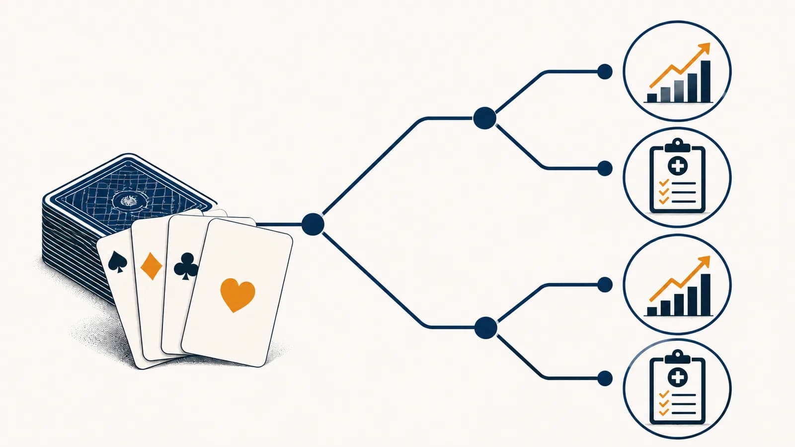
Expected value turns uncertainty into one comparable number
Expected value is the probability weighted average of all possible outcomes of a choice. It is the calculation behind many decisions in poker, venture capital, medicine, insurance, and daily life. By the end, you will be able to calculate expected value, compare uncertain options, and spot situations where the simple answer needs adjusting for risk, missing information, or human consequences.
The idea begins with a list. Write down every outcome you can reasonably identify. Give each outcome a value and a probability. Multiply each value by its probability, then add the products. The result is not a promise about what happens next. It is the average result the same choice would produce across many comparable trials.
For each outcome, multiply its probability by its value , then add every product.
Suppose a fair coin pays you £12 for heads and costs you £8 for tails. Each outcome has probability , so the expected value is . That means an average profit of £2 per play across many plays. You could still lose £8 on the very first flip.
This calculation belongs to the mathematics of probability and uncertainty. Its power comes from separating two questions that people often mix together: “Was the outcome good?” and “Was the decision good given the information available?”
How do you calculate expected value without fooling yourself?
List mutually exclusive outcomes, assign probabilities that add to one, choose a consistent unit of value, multiply, and sum. Then test the assumptions. The arithmetic is usually easy. The difficult work is finding omitted outcomes, realistic probabilities, and values that actually match the decision.
State what you can do now. “Accept the offer” is a choice. “Become successful” is not.
Make the branches cover the realistic possibilities without counting the same event twice.
Use relevant records, base rates, tested models, or clearly stated judgment. Make sure the probabilities total 100%.
Put every outcome in one unit, such as pounds, hours, lives saved, or a carefully defined score.
Calculate the expected value, then change uncertain inputs to see when the preferred choice changes.
Consider two freelance jobs. Job A pays £500 for certain. Job B has a 60% chance of paying £1,000 and a 40% chance of paying nothing because the project might be cancelled. Job A has an expected payment of £500. Job B has an expected payment of . On payment alone, Job B has the higher expected value.
That answer is only as good as the model. Job B may require more hours. Late payment may create fees. The 60% estimate may come from optimism rather than evidence. A sound model adds those effects or displays them as uncertainties. A complicated spreadsheet does not repair imaginary inputs.
One useful check is a break even probability. If Job B pays £1,000 when successful and nothing otherwise, it matches Job A’s £500 expected payment when , so . Above 50%, Job B wins on expected payment. Below 50%, Job A wins. This threshold often helps more than a single confident estimate.
Why can a good decision still produce a bad result?
Expected value judges a decision before uncertainty resolves, using the probabilities and payoffs available then. One outcome judges only what happened afterward. A positive expected value choice can lose, while a reckless choice can get lucky. Results contain evidence, but they do not grade decisions by themselves.
Imagine choosing between a bag with nine winning tickets and one losing ticket, and a second bag with one winning ticket and nine losing tickets. You pick the first bag and draw the loser. The result is bad, but the choice was still better. Reversing the decision because of that one draw would be outcome bias.
“I won, so the decision was smart.” This treats luck as proof and can reward choices with terrible odds.
“Given what I knew, did this choice offer the best probability weighted result?” This keeps the decision and its outcome separate.
The separation works in both directions. A lucky win does not make a poor bet wise. A sensible treatment can fail. A careful investment can lose money. After the result, update the probability estimates if the new evidence is relevant. Do not rewrite what was knowable beforehand.
Repeated decisions make the distinction easier to see. Over many independent trials, observed averages tend to move toward the expected value. Over one trial, almost anything listed in the outcome set can happen. This is why casinos care intensely about a small mathematical edge across many bets, while one visitor can still leave ahead.
There is an important limit. Repetition does not guarantee safety if the trials are dependent, the model is wrong, or one loss ends your ability to continue. A business exposed to the same market shock on every contract does not have thousands of fully separate bets. Counting them as independent makes the risk look smaller than it is.
How do poker players turn cards into a price?
Poker players compare the cost of calling with the probability weighted value of winning the pot. They estimate unseen cards that complete a hand, translate those outs into a chance of success, and compare that chance with the price offered by the pot. Good play follows the calculation repeatedly.
Take a simplified final round. There is £80 in the pot. An opponent bets £20, making the pot £100. You must pay £20 to call. If you call and win, your net gain from this moment is £100. If you lose, your net result is negative £20.
You estimate a 25% chance of winning and a 75% chance of losing. The call has expected value . Under these assumptions, calling earns £10 on average.
The break even winning probability can be found without guessing. A £20 call competes for the £120 total pot that exists after your call. You therefore need to win of the time, or about 16.7%, to break even. An estimated 25% chance is above that threshold.
Real poker adds complications. An opponent may bluff. Your estimate of winning may be wrong. Future betting can change the amount won or lost. Tournament survival can make chips gained and chips lost unequal in practical value. Still, the basic act is clean: convert uncertain cards into probabilities, convert the pot into payoffs, and compare.
This resembles a computing problem. A player narrows a large set of hidden possibilities using visible evidence, much as an efficient method in searching through possible answers avoids checking everything blindly. The human estimate may be rough, but the decision still improves when the assumptions are explicit.
How do venture capitalists price rare successes?
Venture capitalists evaluate portfolios in which many investments may return little and a small number may return far more than the original stake. Expected value forces them to combine each possible company outcome with its probability, rather than treating the most exciting story as the most likely result.
Suppose an investor considers putting £100,000 into a young company. For a transparent teaching example, imagine a 70% chance the stake becomes worth nothing, a 25% chance it becomes worth £200,000, and a 5% chance it becomes worth £2,000,000. The probabilities total 100%.
Against a £100,000 cost, the model gives an expected gain of £50,000 before fees, delay, dilution, taxes, and estimation error.
The rare large outcome contributes £100,000 of the £150,000 expected future value. Remove that branch and the proposal looks poor. This is why the upper tail matters so much in this kind of portfolio. The calculation does not say the company will be worth £150,000. None of the listed outcomes equals that amount.
VC decisions also expose a problem hidden by a positive average: capital is limited. Two investments can each have positive expected value, but the investor may afford only one. Timing matters because money locked up for years cannot fund another opportunity. Ownership can shrink when new shares are issued. Founders and markets can change after the original estimate.
Market structure shapes those assumptions. A company facing several entrenched rivals has different possible payoffs from one protected by strong network effects or high entry costs. The economic tools used to study market power among dominant firms help explain why some optimistic payoff branches are plausible and others are wishful thinking.
How do doctors use expected value without reducing people to money?
Clinical decisions compare uncertain health outcomes, not simply cash returns. Doctors combine evidence about benefits and harms with the patient’s condition and preferences. Expected value can organize the tradeoff, but the chosen value measure must reflect outcomes such as survival, symptoms, side effects, time, and quality of life.
Consider a hypothetical treatment choice. Treatment A gives a modest improvement with a high probability and a mild side effect with a small probability. Treatment B offers a larger possible improvement but also a larger possible harm. Listing those branches prevents attention from settling only on the best outcome or the most frightening one.
A clinical average is not an instruction for one patient. Medical choices depend on diagnosis, individual risk factors, treatment alternatives, evidence quality, and patient preferences. A worked probability example cannot replace advice from a qualified clinician.
Probabilities in medicine often change after a test result. The result must be combined with the condition’s prior probability and the test’s behavior in people with and without the condition. A positive result does not automatically mean the condition is likely. The base rate matters.
Imagine 1,000 people in a deliberately simplified example. Suppose 10 have a condition. A test detects 9 of those 10 and also returns positive for 99 of the 990 people without it. There are 108 positive results, but only 9 are true positives. For a person drawn from this modeled group, the probability of having the condition after a positive result is , about 8.3%.
The figures above are invented inputs for visible arithmetic, not claims about a real disease or test. Their lesson is mechanical: test accuracy and starting prevalence jointly determine what a result means. Doctors then pair the revised probabilities with the consequences of acting, waiting, testing again, or choosing another treatment.
Money can appear in public health decisions because staff time, equipment, and medicines are finite. Yet the value side cannot be reduced to revenue. Health systems may compare health gains, opportunity costs, fairness, and the needs of people who are poorly served by averages. Similar tensions arise in the economics of shared benefits and public goods, where individual payment does not capture all social value.
When does expected value give the wrong practical answer?
Expected value becomes incomplete when losses threaten survival, people value gains and losses unevenly, probabilities are unreliable, outcomes are correlated, or important effects resist a common unit. The calculation may remain arithmetically correct while recommending a choice that a real person or institution cannot safely accept.
A classic example is a bet with a positive average that can bankrupt you. Suppose you have £1,000 and may stake all of it on a 60% chance to gain £1,000, with a 40% chance to lose your entire stake. The expected change is . It is positive. Losing, however, leaves no money for rent, food, or another attempt.
Uses pounds directly and selects the greater probability weighted average amount.
Uses a score for how outcomes affect the decision maker. Losing the last £1,000 can count far more than gaining another £1,000.
Expected utility is one formal response. Instead of placing money itself in the formula, place a utility value that represents the usefulness or harm of each outcome. This explains why paying an insurance premium can be reasonable even when the insurer expects to collect more than it pays out. A predictable small cost may protect against a loss that would be financially devastating.
Uncertain probabilities create another problem. Poker cards come from a defined deck, but a new product, a rare disease, or a geopolitical event may offer little relevant data. A useful response is sensitivity analysis: calculate the result across a range of defensible inputs and find the threshold where the decision changes.
Do not hide uncertainty inside one decimal. If an option wins only when an unsupported estimate is exactly right, the decision is fragile. Show a range, the break even threshold, and the assumptions that drive it.
Some consequences also should not be compressed without discussion. A policy might produce a positive total benefit while concentrating serious harm on a small group. A hospital might improve the average outcome while making access less fair. Expected value can reveal the total modeled effect, but ethical judgment still determines which values belong in the model and which constraints cannot be traded away.
Better decisions come from repeated, revisable estimates
Expected value works best as a disciplined habit: define the choice, expose the branches, estimate honestly, calculate, test the fragile assumptions, and update after new evidence. It does not remove uncertainty. It makes uncertainty visible enough to compare choices without confusing confidence, luck, and wishful thinking.
Before a meaningful decision, write a compact decision record. State the options, probabilities, payoffs, evidence, and conditions that would change your mind. After the outcome, review both the process and the result. A failed prediction may reveal a bad probability estimate, an omitted branch, or ordinary variance. Those explanations call for different changes.
You can spend two hours preparing an application with an estimated 15% chance of producing a £400 opportunity, or use those two hours for work that certainly pays £40. The application has modeled expected value . Its expected advantage is £20, before counting learning, stress, delayed payment, and the reliability of the 15% estimate.
The final choice may still be the certain work. You may need cash today. The £400 outcome may arrive too late. Your estimate may be based on weak evidence. Naming those reasons makes the judgment better, because it shows precisely why the simple expected money result does not settle the choice.
This habit scales. Software teams estimate the chance and cost of failures, economists compare policy outcomes, and households choose warranties or insurance. The models differ, but the questions remain stable: What can happen? How likely is each branch? What is each outcome worth? What could make the estimate wrong?
The takeaway: Choose by expected value when the probabilities and payoffs are credible, then adjust for survival, utility, timing, correlation, fairness, and uncertainty in the model. A good calculation shows its assumptions and survives reasonable changes to them.
Expected value is a cheat code only in the honest sense: it turns vague uncertainty into work you can inspect. It cannot predict the next card, startup, diagnosis, or job offer. It can show which choice is favored by the information you have, what must be true for that answer to hold, and what evidence should change your mind.